DDPM: Denoising Diffusion Probabilistic Models
by MinHyung Lee, UJin Jeong
DDPM: Denoising Diffusion Probabilistic Models
https://arxiv.org/abs/2006.11239
Abstract
Autoregressive, VAE, Normalizing Flow, GAN에서 다양한 장점을 가진 생성모델을 소개하였지만, 이들은 모두 Sampling시간 및 표현력에 있어 각각 단점을 가지고 있었습니다. 우리는 이에 GAN보다 더 좋은 표현력을 가지면서도 어느 정도의 Sampling 속도와 tractable함을 갖춘 Denoising Diffusion Probabilistic Model (DDPM)을 소개합니다.
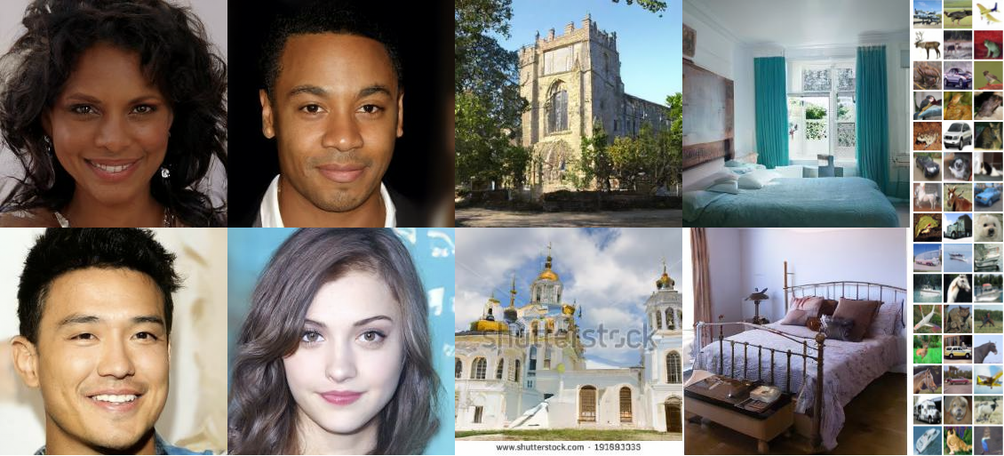
논문에서는 Diffusion probabilistic models을 사용하여 고품질 이미지 합성 결과를 제시합니다. Diffusion probabilistic models과 Langevin dynamics 와의 denoising score matching 사이의 novel connection에 따라 설계된 weighted variational bound에 대한 training을 통해 최상의 결과가 나왔습니다. Unconditional CIFAR10 dataset에서 높은 IS와 FID 를 얻었고 256x256 LSUN에서는 ProgressiveGAN과 유사한 sample quality를 얻었습니다.
출처: (https://github.com/hojonathanho/diffusion)
Code
https://github.com/hojonathanho/diffusion
1. Introduction
Deep generative model인 Generative adversarial networks (GANs), autoregressive models, flows, and variational autoencoders (VAEs)는 이미지 및 오디오 샘플을 합성에서 놀라운 발전이 있었고 최근 다양한 데이터 양식에서 고품질 샘플을 보여주었습니다.
논문에서는 진보된 diffusion probabilistic models을 제안합니다. diffusion probabilistic model (=“diffusion model”)은 유한한 시간 이후 데이터와 matching하는 샘플을 생성하기 위해 variational inference를 사용해 훈련된 parameterized Markov chain 입니다. Chain의 transitions은 signal이 파괴될 때까지 샘플링의 반대 방향으로 데이터에 노이즈를 점진적으로 추가하는 Markov chain인 diffusion process를 reverse하도록 학습됩니다. Diffusion이 small amounts of Gaussian noise로 구성된 경우 sampling chain transitions을 conditional Gaussian으로 설정하면 충분합니다. 특히 simple neural network parameterization 가능합니다. Diffusion models은 정의하기 쉽고 훈련하기에 효율적이지만, 이전까지는, high quality samples을 생성할 수 있다는 증거는 없었습니다. 논문에서는 high quality samples을 생성 가능하고 다른 유형의 생성 모델의 결과와 비교해 때때로 더 나은 성능이 나타남을 보여줍니다. 높은 샘플 품질에도 불구하고 우리 모델은 다른 likelihood-based models 에 비해 경쟁력 있는 log likelihoods를 가지고 있지 않습니다.
2. Background
1. Diffusion Process
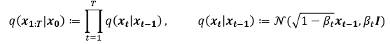
논문에서 사용하는 q는 Diffusion process이며, 이는 아주 미세한 Gaussian noise를 추가하는 과정입니다.
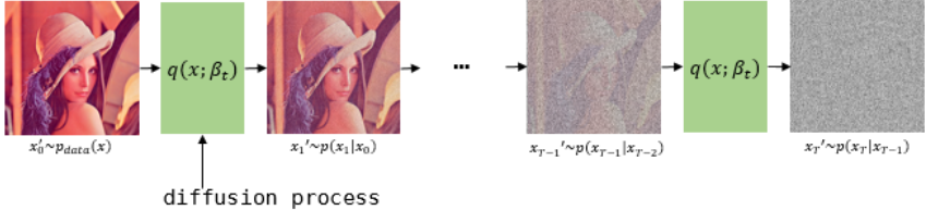
이는 VAE의 경우 Reparametrization trick으로 학습할 수 있으나, 해당 논문에서는 Hyperparameter로 사용하였습니다. 즉 Diffusion process에는 Trainable parameter가 없습니다. 이것을 다회 (해당 Paper에서는 1000회) 반복하여 이미지가 noise화 되는 중간 과정을 Markov chain으로 가정합니다. 즉, 만일 $x_{t-1}$ 이 condition으로 주어진다면 $x_{t-1}$ 이전의 $x_{t-1}, x_{t-3},…$ 에 Independet합니다. $x$ 의 아래첨자는 0~T까지의 Process를 의미하므로, $x_0$ 는 noise가 없는 데이터이고, t가 커짐에 따라 점점 noise가 추가되어 최종 $x_T$ 는 Gaussain noise가 됩니다.
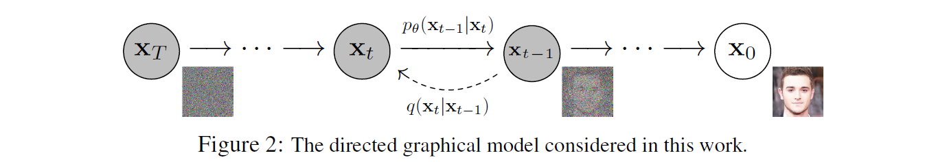
2. Reverse Process
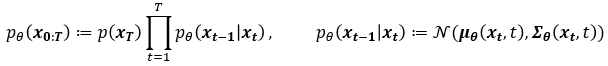
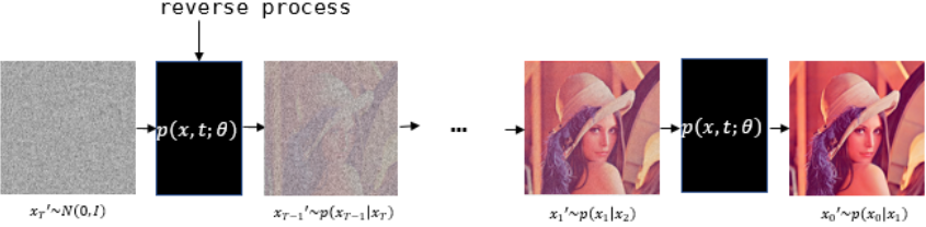
논문에서 표현하는 p는 Reverse process로 Diffusion process와 Gaussian noise $x_T$ 로부터 반대로 미세한 Gaussian noise를 조금씩 걷어내는 과정입니다. 아래 첨자 $\theta$ 를 포함하도록 하여 Neural Network로 학습되는 확률 모델임을 명시합니다. 이 process 또한 Markov cahin입니다.
3. Training Method
DDPM paper의 핵심은 Neural network로 표현되는 p모델이 q를보고 noise를 걷어내는 과정을 하도록 하는 것입니다. 그런데 Diffusion process에서 q는 noise를 매우 미세하게 추가하는 process입니다. noise를 추가하는 것은 gaussian noise로 우리가 직접 추가할 수 있지만, 반대로 걷어내는 과정은 이것이 Gaussain Noise로 가정 될 수 있을지 확실히 알 수 없습니다. 해당 Paper에서는 T가 커져서 Process별 각 단계가 더 세밀화 될 수록 Noise를 걷어내는 과정 역시 Gaussain으로 가정할 수 있다고 표현합니다. 따라서 p를 단순히 q의 $\mu (mean), \sigma(std)$와 같아지도록 학습한다면 p 또한 당연히 noise가 추가되는 process로 자연스럽게 학습이 가능해집니다.


4. Diffusion models and denoising autoencoders mathematical expression
DDPM은 어떻게보면 Hierachical VAE로 볼 수 있기에, DDPM Loss를 설명하기 위해 VAE Loss의 유도과정을 먼저 간단히 되짚어 보겠습니다. Ref)https://lilianweng.github.io/posts/2021-07-11-diffusion-models/
1. VAE Loss
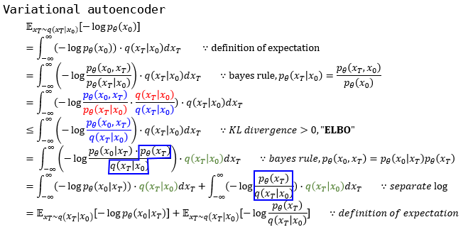
VAE에서 latent는 z로 표현함으로 $x_T$를 z로 치환하면 기존에 보던 식이 됩니다. 위 수식에서 알수 있듯, VAE에서 수식을 전개할때 사용하는 트릭은,
- ${q(x_T|x_0) \over q(x_T|x_0)}$ 를 곱해줌으로써 intractable KL divergence를 없애, ELBO로 표현하기
- ELBO 수식에서 bayseian표현으로 갈라져나온 $p_\theta(x_T)$가 Latent의 KL Divergence
- ELBO 수식에서 Latent KL divergence를 제외한 나머지가 Reconstruction term으로 남아 두 Loss term으로 표현 가능으로 정리됩니다.
2. DDPM Loss
VAE의 loss를 구하는 방식을 DDPM에 적용해보겠습니다.
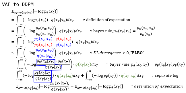
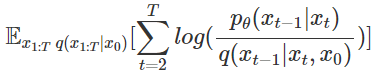
DDPM에서는 ELBO 식의 분모가 Latent의 KL divergence loss가 되도록 붙이는 것이 아니라 VAE에서 Reconstruction term이 되는 분자와 합치게 됩니다. 결국 맨 아래 수식을 보면 $p_\theta(x_0|x_T)$ 와 $q(x_T|x_0)$ 의 KL divergence를 최소화 하도록 합니다.
그렇다면, Training Method에서 이야기했던 q로부터 어떻게 p를 학습 시킬 것이냐는 것은 아래 수식으로 풀 수 있습니다. 이것에 대한 간략한 Key는 두 분포의 Condition과 Target variable이 서로 반대라는 것입니다.
3. Intractable → Tractable
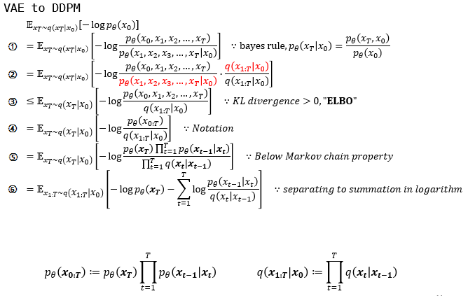
①: bayes rule을 바탕으로 multi-variable에 대한 conditional, joint probability로 나누었습니다.
②: VAE에서 쓰인 트릭처럼 ${q(x_T|x_0) \over q(x_T|x_0)}$ 를 곱해줍니다.
③: ②에서 빨간색으로 표현된 부분을 intractable한 KL divergence term으로 제거하고 ELBO를 남깁니다.
⑤: p와 q가 markov chain임을 이용하여 Markov chain의 성질을 이용하여 $\prod$ 로 표현하였습니다.
⑥: log의 성질로 곱으로 표현된 부분을 합으로 나타내었습니다.
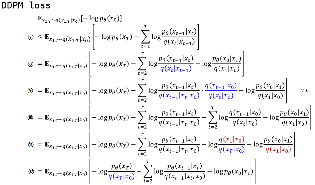
⑧: $\sum$의 아래첨자의 t가 2가 되고 $\sum$ 첫 번째 term을 뒤로 따로 빼냈습니다.
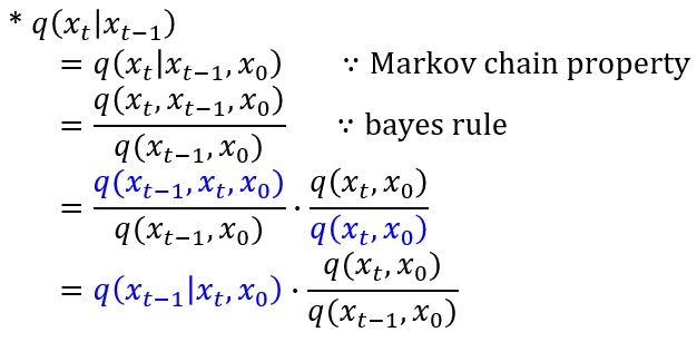
⑨: Markov chain의 성질로 나타낼 수 있는 부분입니다. 사실상 loss term을 만들어낼 때 제일 핵심이 되는 구간이라고 생각합니다. 이 과정을 통해서 수식 내의 p와 q distribution이 같은 condition으로부터 같은 target distribution을 나타내게 되었습니다.
⑩: log의 성질로 곱으로 표현된 부분을 합으로 나타내었습니다.
⑪: ⑩에서 log로 갈라져나온 term을 보면 t=i에서의 분모가 t=i+1에서의 분자와 약분됩니다.
⑫: ⑪에 파란색 분모부분을 앞으로 빼고 남은 term을 정리해서 남겨놓습니다.
4. Loss Term의 의미
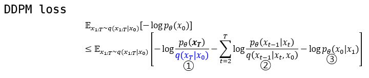
①: p가 만드는 noise $x_T$ 의 분포와 data $x_0$ 로부터 q과정을 거쳐 만들어진 noise $x_T$ 의 분포간 KL divergence를 최소화합니다. 이 loss는 process를 매우 많이 진행하여 분모의 분포가 $x_T$ 가 $x_0$ 와 independent한 Gaussian distribution라고 가정하여 p 또한 그냥 Gaussian distribution에서 sampling하는 방식을 취하여 이 term에 의해서는 Neural net은 학습되지 않습니다.
②: latent상에서 $x_t$ 로부터 $x_{t-1}$ 의 분포를 예측하는 reverse process는 q가 Gaussian process일 경우 아래의 수식으로 나타낼 수 있습니다.
③: VAE의 reconstruction loss와 같은 역할을 합니다. latent $x_1$ 로부터 data인 $x_0$ 을 추정하는 확률 모델의 parameter를 최적화시킵니다.
다시 정리해보면,
①은 VAE의 KL divergence와 비슷한 term이고,
②는 reverse process와 diffusion process의 분포를 매칭시키는(KL divergence를 낮추는) loss이고
③은 reverse process의 마지막 과정으로, VAE의 reconstruction loss에 대응되는 term이라고 볼 수 있습니다.
5. Training technique
1) Latent $p_\theta(x_T)$ 가 $q(x_T|x_0)$ 와 가까워 지도록 변경
Paper에서는 noise schedule $\beta$ 에 대해 아래처럼 정의합니다.
” ${\beta_t}$ 가 학습가능하긴 한데, 우리는 constant로 뒀다. 그래서 q는 learnable parameters가 아니라 Neural net으로 학습시키지 않는다. 그러므로 ①번 loss는 constant로 학습과정에서 제외된다.”
실제로 논문의 내용을 확인하면 $\beta_{1} = 10^{-4}$ 에서 $\beta_{T}=0.02$ 까지 T=1000 으로 linear하게 증가한다고 하며, 이 정보에 따라 $q(x_{T}|x_{0})$ 를 계산해보면, $q(x_T|x_0) =$ $N(x_T;0.00635x_0, 0.99995I)$ 로 거의 $N(0, I)$ 에 가까워집니다. 즉 noise latent $x_{T}$ 를 얻을때 VAE와 같이 따로 어떤 분포를 따라갈 필요가 없이 $x_{T}$ 의 sampling은 Gaussian distribution에서 sampling하게 됩니다.
2) ② reverse process가 diffusion process와의 KL divergence가 낮게, 그리고 학습 시 technique
이전 포스트에서 diffusion process와 reverse process가 서로 condition과 target variable이 교차되어 있지만 수식 전개를 통해 condition, target variable을 matching시켜주었습니다.
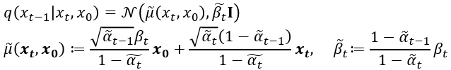
위 Term에서 log의 분모 $q(x_{t-1}|x_t, x_0)$ 는 $q(x_{t-1}|x_t,x_0) = N(\widetilde{\mu}(x_t,x_0), \tilde{\beta_t}I)$ 로

tractable하게 구할수 있습니다. Neural net으로 model 선언시 확률모델을 설계하면 output으로 $\mu_\theta, \sigma_\theta$를 추정하게 되는데, 여기서 $\mu_\theta$는 위의 $\widetilde{\mu}(x_t,x_0)$와 가까워지도록 학습하게 됩니다. 여기서 $x_t를 x_0$에 대한 reparametrization 형태로 나타내고 식을 정리하면
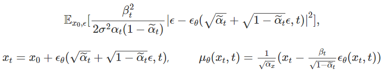
가 되고, Loss식을 보게 되면 Neural net의 output $\epsilon_\theta$이 Gaussain $\epsilon$과의 Mean squaare error를 최소화 하도록 optimize하게 됩니다.
최종적으로 Paper에서는 optimize할 위의 식보다 Coefficient인자들을 뺀
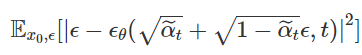
를 Update하는 것이 생성모델 성능이 더 좋았다고 설명합니다. 그 이유는 loss의 coefficient는 t가 증가함에 따라 작아집니다. 따라서 coefficient를 제거하면 t가 큰 process의 loss가 상대적으로 더 커진 것과 같으므로 larger t의 process에 더 집중하게 됩니다. 논문에서는 학습의 입장에서도 이미지에 가까운(덜 noisy한) 것에서 noise를 제거하는 것보다 noise가 심한 이미지에서 noise를 제거하는 것에 더 집중하는 모델이 성능이 좋을 것이라고 설명하였습니다.
3) ③마지막 latent $x_{1}$ 에서 data $x_{0}$ 로의 Reconstruction
VAE에서는 Gaussian $z\sim \mathcal{N}(0, I)$ 에서 image로 Reconstruction이었다면 DDPM의 Reconstruction은 아주 미세하게(one-process-infinitesimally) noisy한 이미지에서 원래의 image로의 Reconstruction이므로 학습되는 Task라고 할 수 있습니다. 수식으로 표현하면,
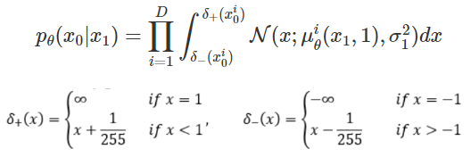
로서, 실제 구현 상에서는 이미지 $x_0$에 대해 $x_1$을 집어넣어 나온 결과가 $x_0$와의 MSE Loss를 최소화 하는 것과 같습니다.
5. Experiments
Sample quality
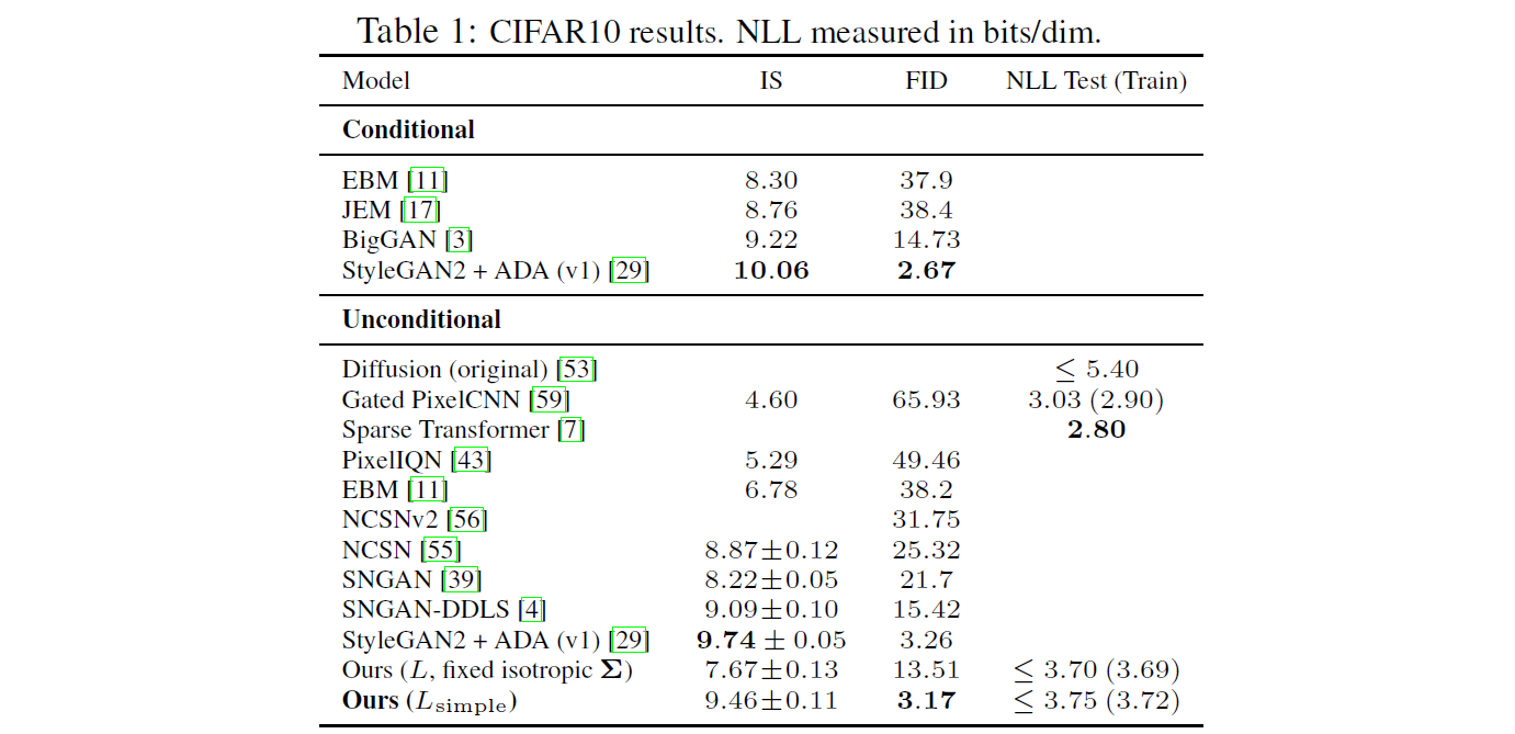
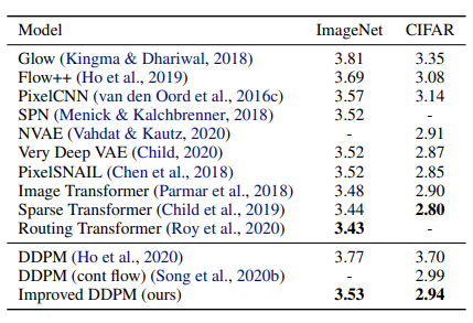
Table 1은 CIFAR 10의 Inception score, FID score, Negative Log Likelihoods 를 보여줍니다.
FID (train set) : 3.17 & FID (test set) : 5.24
DDPM은 Unconditional한 경우 중에서 가장 높은 sample quality 를 보입니다.
Ours $(L_{simple})$ (즉, 계수 Term을 제외한 경우)와 Ours $(L,$ $fixed$ $isotropic$ $Σ)$ (즉, 계수 Term을 제외하지 않은 경우)를 비교하면, Ours $(L_{simple})$ 에서 NLL이 다소 낮은 성능을 보이지만, FID score에서는 큰 향상을 보이는 것을 확인할 수 있습니다.
Reverse process parameterization and training objective ablation
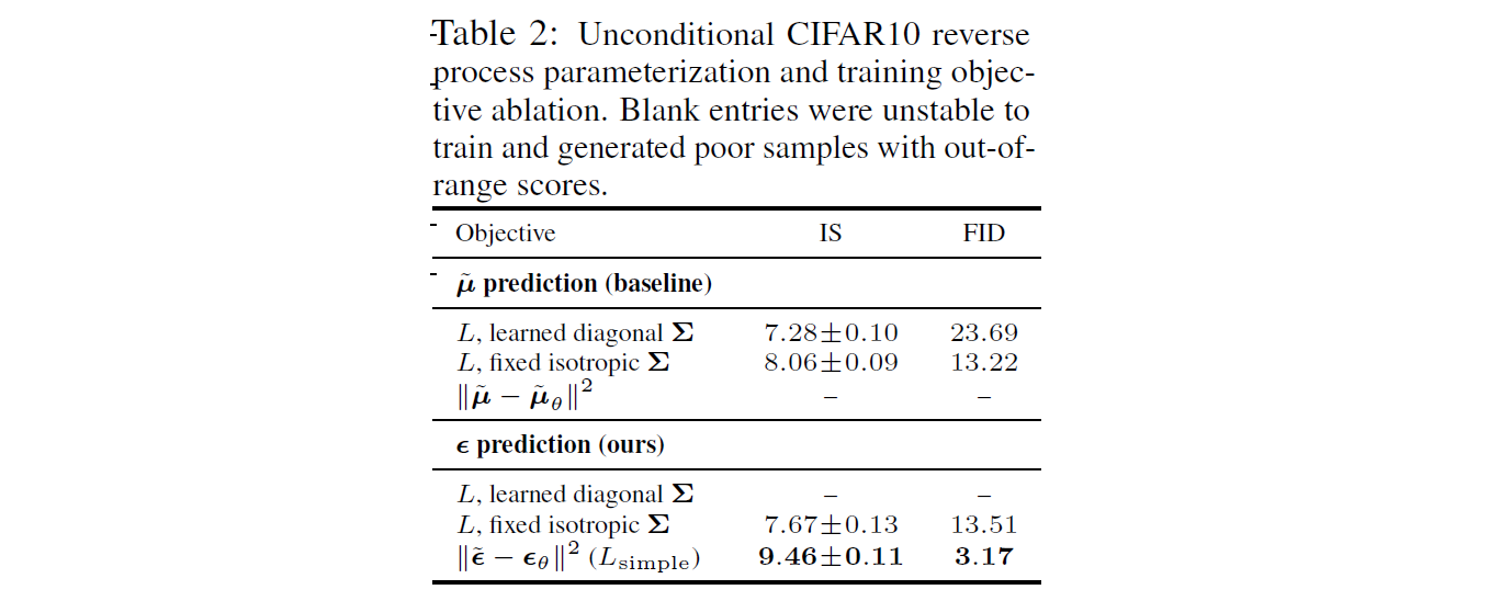
Table2에서는 reverse process parameterization 과 training objectives 의 sample quality effects를 보여줍니다.
$\tilde{μ}$ prediction:
- 학습한 경우보다 Fixed variance를 사용한 경우, 성능이 향상되었습니다.
- simplified objective를 사용한 경우, 성능이 악화 되었습니다.
ε prediction:
- Reverse process variances를 학습하는 것이 훈련의 불안정성을 초래해 fixed variance에 비해 sample quality가 저하된다는 것을 알 수 있습니다.
- Fixed variance를 사용한 경우, $\tilde{μ}$ 를 예측하는 것과 거의 비슷한 성능을 보였습니다.
- Simplified objective를 사용해 훈련을 한 경우 성능이 향상되었습니다.
- 참고: (표에서 - 는 성능이 매우 악화되었다는 의미입니다.)
결론적으로, $\tilde{μ}$ prediction 보다는 ε prediction에서 더 높은 성능을 보였습니다.
Progressive generation
Figture 6 and 10은 reverse process 동안 $\hat{x_{0}}$ 의 sample quality 결과를 보여줍니다.
Large scale image feature가 먼저 나타나고 details는 나중에 나타나는 것을 확인 가능합니다.
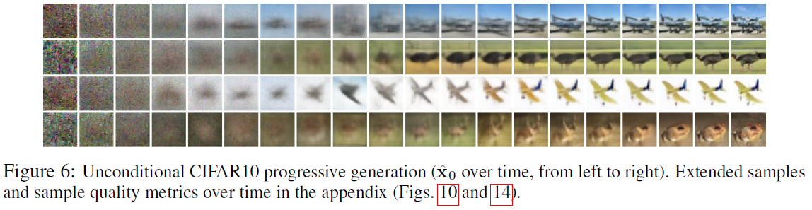
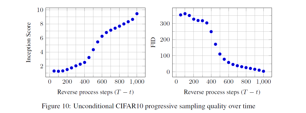
Figure 7은 various t에 대해 $x_t$ 가 frozen된 stochastic prediction $x_0$ ~ $p_θ(x_0|x_t)$ 를 보여줍니다.
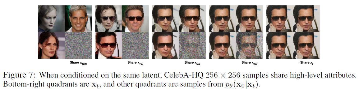
t(small): fine detail을 제외하고는 모두 보존됩니다.
t(large): large scale features만 보존됩니다.
6. Conclusion
Strong Points
- GAN에 못지 않은 high quality sample을 생성 가능합니다.
- GAN의 단점인 mode collapse에 빠지지 않습니다.
- Latent vactor를 사용해서 data를 잘 압축할 수 있습니다.
- Explict하게 표현 가능한 모델입니다.
Weak Points
- Sampling을 진행할 때마다 reverse step(T)을 거쳐야 하기 때문에 Sampling 시간이 길다는 단점이 있습니다.
Autoregressive, VAE, Normalizing Flow, GAN 외에도 Generative model에 새로운 선택지를 제시했다는 점에서 의의가 있다고 생각합니다. 추가로 Diffusion models은 이미지 데이터에 대한 우수한 inductive biases을 가지고 있는 것으로 보이므로, 다른 데이터 양식과 다른 유형의 생성 모델 및 기계 학습 시스템의 구성 요소로서의 더 활용을 기대한다고 합니다.
Broader Impact
Diffusion models에 대한 해당 논문의 연구는 GANs, flows, autoregressive models 등의 sample quality를 개선하기 위한 노력과 같은 다른 유형의 deep generative models에 대한 기존 작업과 유사한 범위를 갖습니다.
해당 논문은 diffusion models을 이 기술 계열에서 일반적으로 유용한 도구로 만드는 데 있어 progress를 나타내므로, generative models이 broader world에서 가지는 영향력을 증폭시키는 역할을 할 수 있습니다.
부정적 영향
-
악의적인 사용 사례
생성 모델의 잘 알려진 많은 악의적인 사용 사례들이 있습니다. 예를 들어, Sample generation 기술을 사용하여 정치적 목적을 위한 유명 인사들의 fake 이미지와 비디오를 생성할 수 있습니다.
Fake 이미지는 이전에는 수동으로 만들어졌지만, 생성 모델의 발전으로 fake 이미지를 만드는 것이 더 쉬워졌습니다.
다행히, CNN-generated 이미지는 현재 탐지를 허용하는 미묘한 결함을 가지고 있지만, 생성 모델의 발전으로 인해 이것이 더 어려워질 수 있습니다.
-
편향된 training data
생성 모델은 training 데이터 세트의 biases를 반영합니다.
자동화 된 시스템에 의해 인터넷에서 많은 대규모 데이터 세트가 수집되기 때문에, 특히 이미지에 레이블이 지정되지 않은 경우에는 이러한 biases을 제거하는 것이 어려울 수 있습니다.
이러한 데이터 세트에 대해 훈련된 생성 모델의 샘플이 인터넷 전체에 확산되면, 이러한 편향은 더욱 강화될 수 있습니다.
긍정적 영향
-
데이터 압축
반면에, diffusion models은 데이터 압축에 유용할 수 있습니다.
데이터가 더 높은 해상도가 되고, 글로벌 인터넷 트래픽이 증가함에 따라 광범위한 사용자들에게 인터넷의 접근성을 보장하는 데 중요하게 작용할 수 있습니다.
-
AI 학습
Image classification에서 reinforcement learning에 이르기까지 광범위한 downstream 작업을 위해 레이블이 지정되지 않은 raw data에 대한 representation learning에 기여할 수 있습니다.
-
창의적인 용도의 사용
Diffusion models은 예술, 사진 및 음악에서 창의적인 용도로 사용하게 될 수 있습니다.
7. Future work
Improved DDPM: Improved Denoising Diffusion Probabilistic Models
https://arxiv.org/abs/2102.09672
Improved DDPM에서 제시하는 바는 다음과 같습니다.
- Improving log-likelihood
- Learning $\Sigma_\theta (x_t, t)$
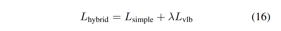
- Parameterization 및 $L_{hybrid}$ objective (hybrid loss term)를 사용해 $Σ_θ$ 를 학습하면 이전보다 competitive한 log-likelihood를 갖게 됩니다.
- 조금 더 자세히 설명하자면, DDPM에서는 β 값을 constant로 사용했으나, 이를 parameterization을 통해 optimal한 값을 찾으려고 했습니다.
- 또한, DDPM에서는 $L_{simple}$ 만 사용했으나, Improved DDPM에서는 loss term을 추가해 $L_{hybrid}$ 로 학습을 진행했습니다. (λ는 hyper parameter)

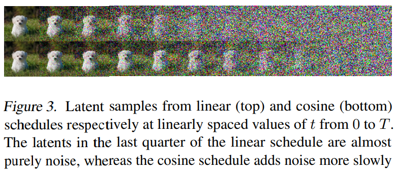
- Improving the Noise Schedule (linear → cosine)
- Linear schedule 대신 cosine schedule을 사용했습니다.
- Reducing Gradient Noise (importance sampling)
- Importance sampling 을 통해 Gradient Noise를 줄였습니다.
- Learning $\Sigma_\theta (x_t, t)$
- Reduced sampling step
- Sampling 시 training 할 때보다 더 적은 diffusion step 사용했습니다.
- Comparision to GAN
- GAN의 sample quality와 유사하면서 recall을 측정했을 때 훨씬 더 나은 mode coverage를 달성할 수 있다는 것을 발견했습니다.
- Scaling Model Size
- Model의 sample quality와 log-likelihood가 model capacity 및 training compute에 따라 부드럽게 확장할 수 있음을 보여줍니다.
요약하자면, 기존 DDPM은 image quality가 높았지만 log-likelihood의 수치는 그다지 좋지 못했습니다. Improved DDPM에서는 이를 해결하기 위해 더 나은 noise schedule을 사용하고, 기존의 loss에 추가 loss term을 붙인 hybrid loss term을 제안했습니다.
또한, sampling step에도 변화를 주어 기존 DDPM 보다 더 빠르게 샘플링이 가능하게 했습니다.
결과적으로, 샘플 품질에 거의 영향을 미치지 않으면서 빠른 샘플링이 가능하고 더 나은 log likelihood가 나오는 모델을 선보였습니다.
Improved DDPM에서 사용된 이미지 출처: (https://arxiv.org/abs/2102.09672)
DDIM: DENOISING DIFFUSION IMPLICIT MODELS
https://arxiv.org/abs/2010.02502
DDPM은 adversarial training 없이 high quality image를 generation 했습니다. 그러나, 모델을 학습하고 추론하는 과정에서 sample을 생성하기 위해 많은 steps에서 Markov chain을 simulating해야 한다는 문제가 있습니다.
DDIM에서는 보다 빠른 samping을 위해 non-Markovian diffusion process을 이용해 DDPM을 일반화했습니다. non-Markovian diffusion process를 통해 deterministic한 generative processes를 수행 가능하게 되었습니다. DDIM은 DDPM에 비해 high quality sample을 10배에서 50배 정도 더 빨리 생산 가능합니다.
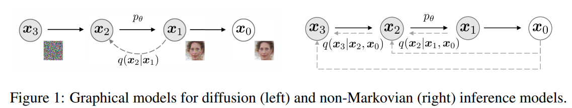
DDPM:

DDIM:

DDPM은 $x_t$ 가 이전 step 인 $x_{t-1}$ 에 의해 결정되는 markov chain입니다.
DDIM은 $x_t$ 가 이전 step 인 $x_{t-1}$ 와 $x_{0}$ 에 의해 결정되는 non-markov chain입니다.
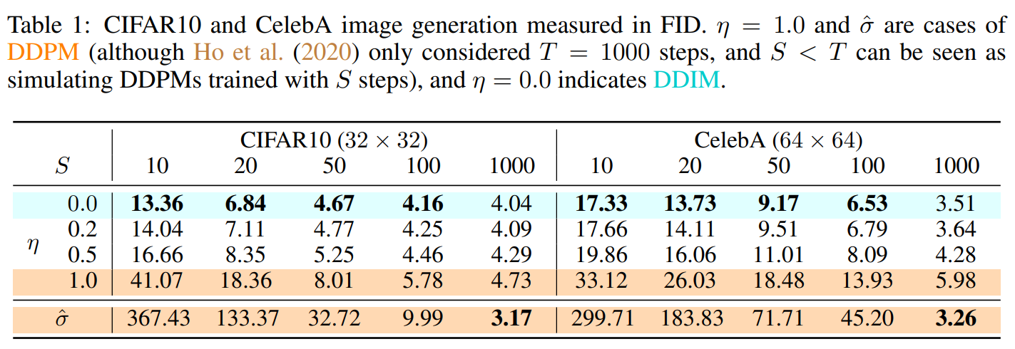
Table 1을 보면, DDIM이 DDPM보다 전반적으로 높은 성능을 보이는 것을 확인 가능합니다.
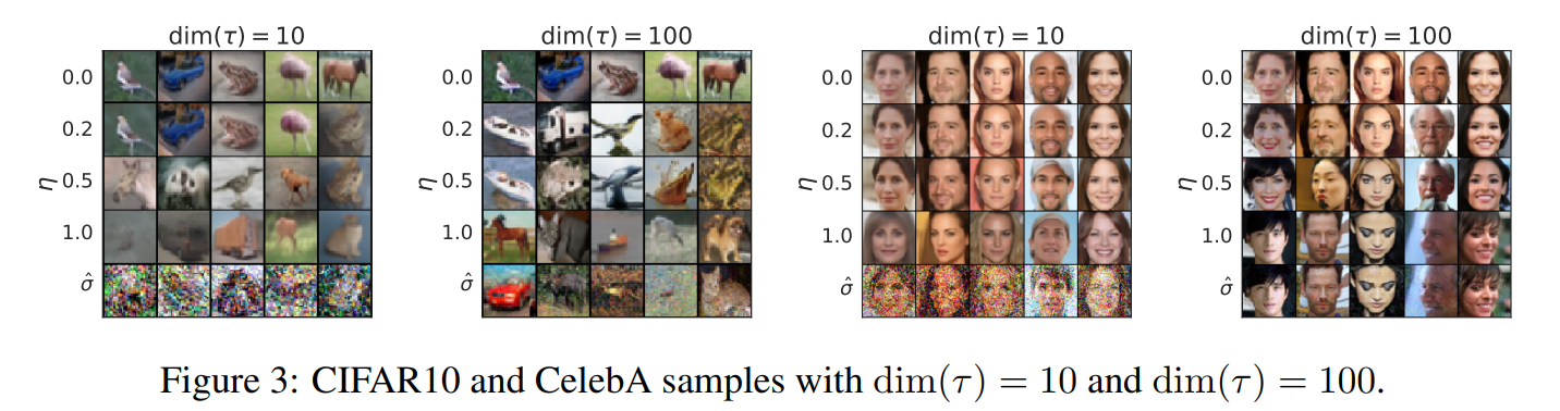
Figure 3를 보면, dim이 커질수록 sample quality가 좋아집니다. (단, computational cost는 증가합니다.)
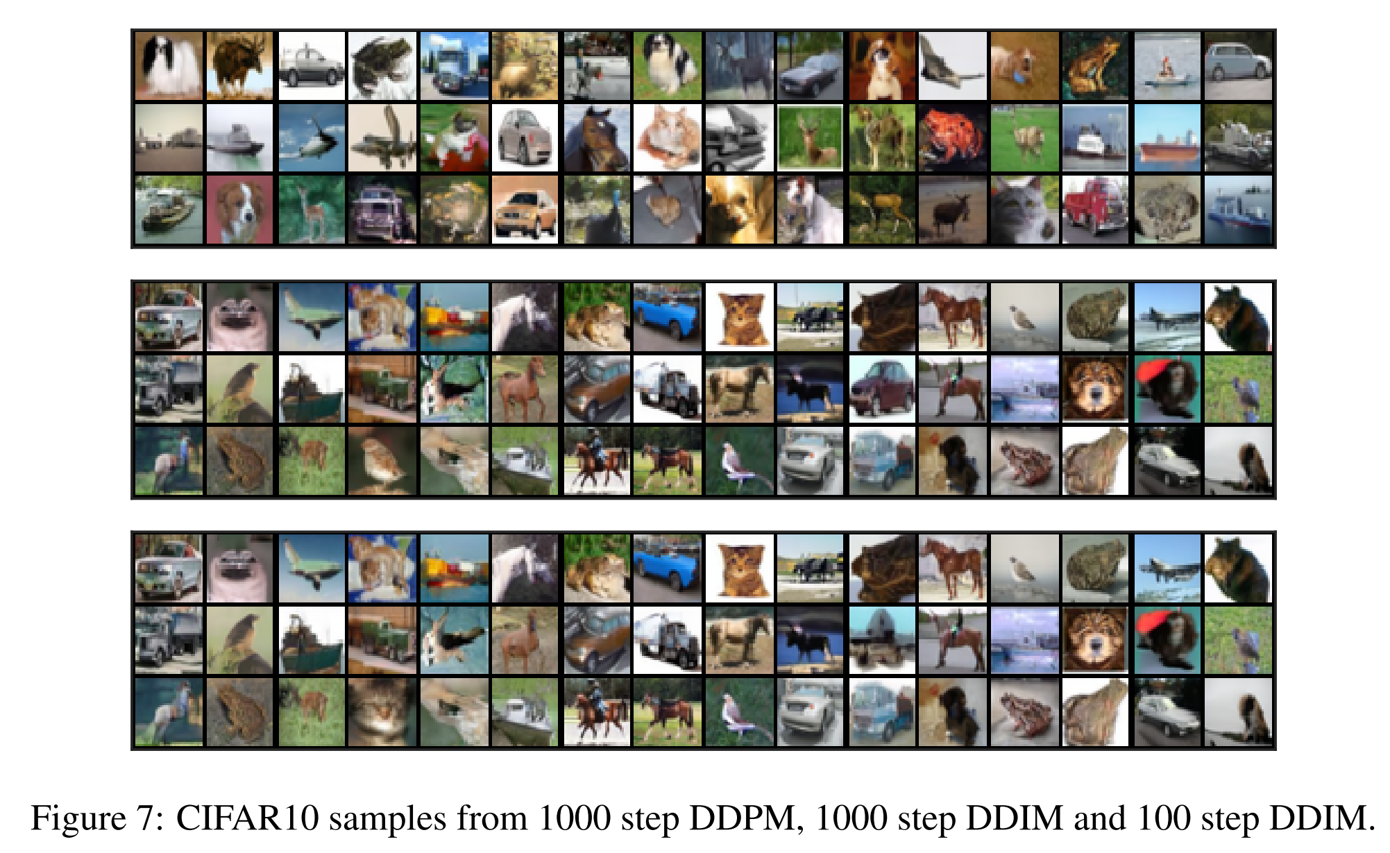
Figure 7을 보면, 기존에 DDPM으로는 1000 step 정도 거쳐야 얻을 수 있었던 결과를 DDIM에서는 100 step 정도만 진행해도 유사한 결과를 얻을 수 있는 것을 확인할 수 있습니다.
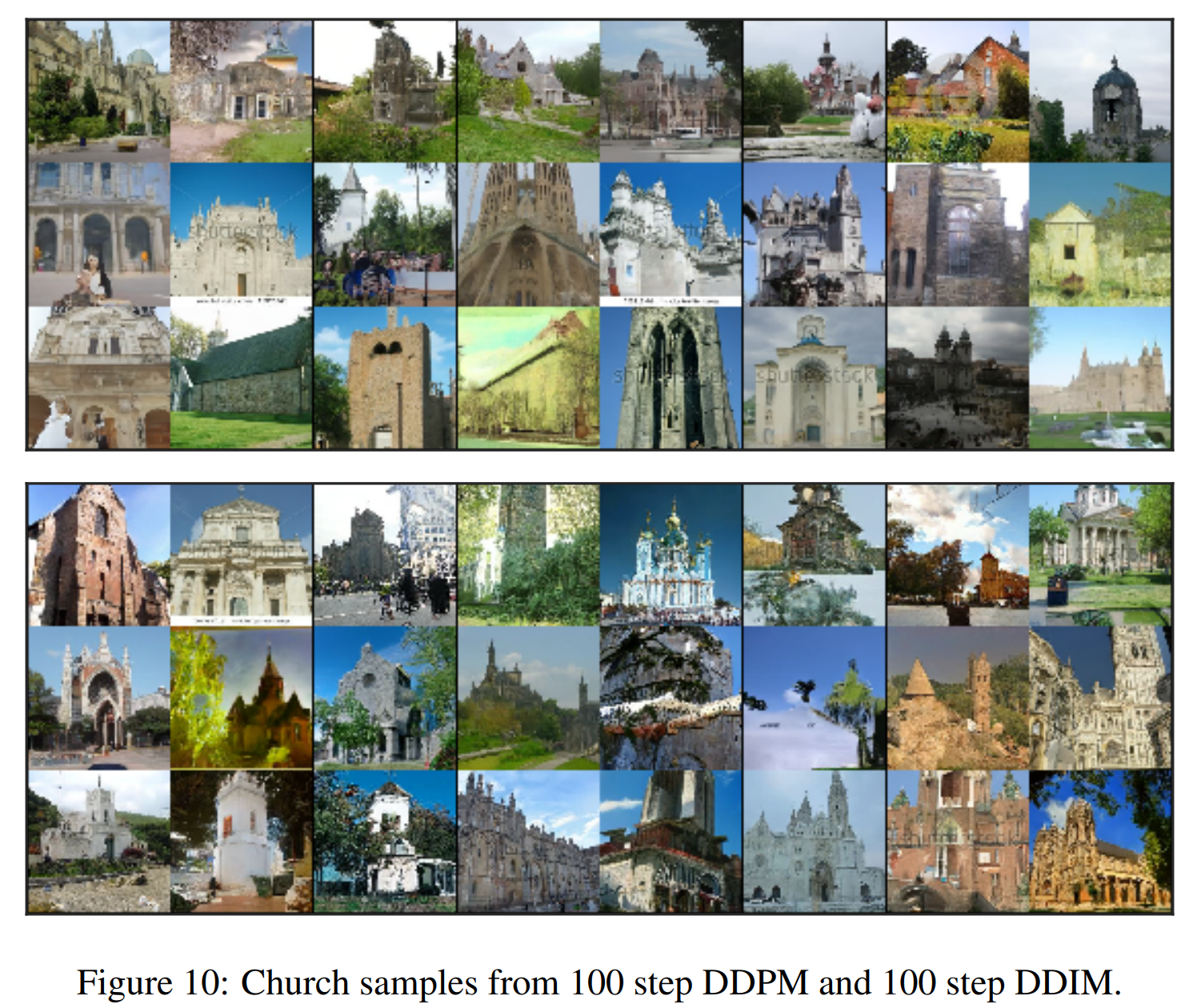
Figure 10을 보면, 같은 100 step의 DDPM과 DDIM을 비교한 이미지입니다.
대략적인 이미지만 본다면 DDPM도 꽤 괜찮은 성능을 보이는 것처럼 보이나, detail한 부분에서 차이가 나는 것을 확인할 수 있습니다.
DDIM에서 사용된 이미지 출처: (https://arxiv.org/abs/2010.02502)
Code - Main function : Beta Schedule / Gaussian Diffusion
      class GaussianDiffusion:


        def __init__(self, *, betas, loss_type, tf_dtype=tf.float32):
          self.loss_type = loss_type

          assert isinstance(betas, np.ndarray)
          self.np_betas = betas = betas.astype(np.float64)  # computations here in float64 for accuracy
          assert (betas > 0).all() and (betas <= 1).all()
          timesteps, = betas.shape
          self.num_timesteps = int(timesteps)

          alphas = 1. - betas
          alphas_cumprod = np.cumprod(alphas, axis=0)
          alphas_cumprod_prev = np.append(1., alphas_cumprod[:-1])
          assert alphas_cumprod_prev.shape == (timesteps,)

          self.betas = tf.constant(betas, dtype=tf_dtype)
          self.alphas_cumprod = tf.constant(alphas_cumprod, dtype=tf_dtype)
          self.alphas_cumprod_prev = tf.constant(alphas_cumprod_prev, dtype=tf_dtype)

          # calculations for diffusion q(x_t | x_{t-1}) and others
          self.sqrt_alphas_cumprod = tf.constant(np.sqrt(alphas_cumprod), dtype=tf_dtype)
          self.sqrt_one_minus_alphas_cumprod = tf.constant(np.sqrt(1. - alphas_cumprod), dtype=tf_dtype)
          self.log_one_minus_alphas_cumprod = tf.constant(np.log(1. - alphas_cumprod), dtype=tf_dtype)
          self.sqrt_recip_alphas_cumprod = tf.constant(np.sqrt(1. / alphas_cumprod), dtype=tf_dtype)
          self.sqrt_recipm1_alphas_cumprod = tf.constant(np.sqrt(1. / alphas_cumprod - 1), dtype=tf_dtype)

          # calculations for posterior q(x_{t-1} | x_t, x_0)
          posterior_variance = betas * (1. - alphas_cumprod_prev) / (1. - alphas_cumprod)
          # above: equal to 1. / (1. / (1. - alpha_cumprod_tm1) + alpha_t / beta_t)
          self.posterior_variance = tf.constant(posterior_variance, dtype=tf_dtype)
          # below: log calculation clipped because the posterior variance is 0 at the beginning of the diffusion chain
          self.posterior_log_variance_clipped = tf.constant(np.log(np.maximum(posterior_variance, 1e-20)), dtype=tf_dtype)
          self.posterior_mean_coef1 = tf.constant(
            betas * np.sqrt(alphas_cumprod_prev) / (1. - alphas_cumprod), dtype=tf_dtype)
          self.posterior_mean_coef2 = tf.constant(
            (1. - alphas_cumprod_prev) * np.sqrt(alphas) / (1. - alphas_cumprod), dtype=tf_dtype)

        @staticmethod
        def _extract(a, t, x_shape):
          """
          Extract some coefficients at specified timesteps,
          then reshape to [batch_size, 1, 1, 1, 1, ...] for broadcasting purposes.
          """
          bs, = t.shape
          assert x_shape[0] == bs
          out = tf.gather(a, t)
          assert out.shape == [bs]
          return tf.reshape(out, [bs] + ((len(x_shape) - 1) * [1]))

        def q_mean_variance(self, x_start, t):
          mean = self._extract(self.sqrt_alphas_cumprod, t, x_start.shape) * x_start
          variance = self._extract(1. - self.alphas_cumprod, t, x_start.shape)
          log_variance = self._extract(self.log_one_minus_alphas_cumprod, t, x_start.shape)
          return mean, variance, log_variance

        def q_sample(self, x_start, t, noise=None):
          """
          Diffuse the data (t == 0 means diffused for 1 step)
          """
          if noise is None:
            noise = tf.random_normal(shape=x_start.shape)
          assert noise.shape == x_start.shape
          return (
              self._extract(self.sqrt_alphas_cumprod, t, x_start.shape) * x_start +
              self._extract(self.sqrt_one_minus_alphas_cumprod, t, x_start.shape) * noise
          )

        def predict_start_from_noise(self, x_t, t, noise):
          assert x_t.shape == noise.shape
          return (
              self._extract(self.sqrt_recip_alphas_cumprod, t, x_t.shape) * x_t -
              self._extract(self.sqrt_recipm1_alphas_cumprod, t, x_t.shape) * noise
          )

        def q_posterior(self, x_start, x_t, t):
          """
          Compute the mean and variance of the diffusion posterior q(x_{t-1} | x_t, x_0)
          """
          assert x_start.shape == x_t.shape
          posterior_mean = (
              self._extract(self.posterior_mean_coef1, t, x_t.shape) * x_start +
              self._extract(self.posterior_mean_coef2, t, x_t.shape) * x_t
          )
          posterior_variance = self._extract(self.posterior_variance, t, x_t.shape)
          posterior_log_variance_clipped = self._extract(self.posterior_log_variance_clipped, t, x_t.shape)
          assert (posterior_mean.shape[0] == posterior_variance.shape[0] == posterior_log_variance_clipped.shape[0] ==
                  x_start.shape[0])
          return posterior_mean, posterior_variance, posterior_log_variance_clipped

        def p_losses(self, denoise_fn, x_start, t, noise=None):
          """
          Training loss calculation
          """
          B, H, W, C = x_start.shape.as_list()
          assert t.shape == [B]

          if noise is None:
            noise = tf.random_normal(shape=x_start.shape, dtype=x_start.dtype)
          assert noise.shape == x_start.shape and noise.dtype == x_start.dtype
          x_noisy = self.q_sample(x_start=x_start, t=t, noise=noise)
          x_recon = denoise_fn(x_noisy, t)
          assert x_noisy.shape == x_start.shape
          assert x_recon.shape[:3] == [B, H, W] and len(x_recon.shape) == 4

          if self.loss_type == 'noisepred':
            # predict the noise instead of x_start. seems to be weighted naturally like SNR
            assert x_recon.shape == x_start.shape
            losses = nn.meanflat(tf.squared_difference(noise, x_recon))
          else:
            raise NotImplementedError(self.loss_type)

          assert losses.shape == [B]
          return losses

        def p_mean_variance(self, denoise_fn, *, x, t, clip_denoised: bool):
          if self.loss_type == 'noisepred':
            x_recon = self.predict_start_from_noise(x, t=t, noise=denoise_fn(x, t))
          else:
            raise NotImplementedError(self.loss_type)

          if clip_denoised:
            x_recon = tf.clip_by_value(x_recon, -1., 1.)

          model_mean, posterior_variance, posterior_log_variance = self.q_posterior(x_start=x_recon, x_t=x, t=t)
          assert model_mean.shape == x_recon.shape == x.shape
          assert posterior_variance.shape == posterior_log_variance.shape == [x.shape[0], 1, 1, 1]
          return model_mean, posterior_variance, posterior_log_variance

        def p_sample(self, denoise_fn, *, x, t, noise_fn, clip_denoised=True, repeat_noise=False):
          """
          Sample from the model
          """
          model_mean, _, model_log_variance = self.p_mean_variance(denoise_fn, x=x, t=t, clip_denoised=clip_denoised)
          noise = noise_like(x.shape, noise_fn, repeat_noise)
          assert noise.shape == x.shape
          # no noise when t == 0
          nonzero_mask = tf.reshape(1 - tf.cast(tf.equal(t, 0), tf.float32), [x.shape[0]] + [1] * (len(x.shape) - 1))
          return model_mean + nonzero_mask * tf.exp(0.5 * model_log_variance) * noise

        def p_sample_loop(self, denoise_fn, *, shape, noise_fn=tf.random_normal):
          """
          Generate samples
          """
          i_0 = tf.constant(self.num_timesteps - 1, dtype=tf.int32)
          assert isinstance(shape, (tuple, list))
          img_0 = noise_fn(shape=shape, dtype=tf.float32)
          _, img_final = tf.while_loop(
            cond=lambda i_, _: tf.greater_equal(i_, 0),
            body=lambda i_, img_: [
              i_ - 1,
              self.p_sample(denoise_fn=denoise_fn, x=img_, t=tf.fill([shape[0]], i_), noise_fn=noise_fn)
            ],
            loop_vars=[i_0, img_0],
            shape_invariants=[i_0.shape, img_0.shape],
            back_prop=False
          )
          assert img_final.shape == shape
          return img_final

        def p_sample_loop_trajectory(self, denoise_fn, *, shape, noise_fn=tf.random_normal, repeat_noise_steps=-1):
          """
          Generate samples, returning intermediate images
          Useful for visualizing how denoised images evolve over time
          Args:
            repeat_noise_steps (int): Number of denoising timesteps in which the same noise
              is used across the batch. If >= 0, the initial noise is the same for all batch elemements.
          """
          i_0 = tf.constant(self.num_timesteps - 1, dtype=tf.int32)
          assert isinstance(shape, (tuple, list))
          img_0 = noise_like(shape, noise_fn, repeat_noise_steps >= 0)
          times = tf.Variable([i_0])
          imgs = tf.Variable([img_0])
          # Steps with repeated noise
          times, imgs = tf.while_loop(
            cond=lambda times_, _: tf.less_equal(self.num_timesteps - times_[-1], repeat_noise_steps),
            body=lambda times_, imgs_: [
              tf.concat([times_, [times_[-1] - 1]], 0),
              tf.concat([imgs_, [self.p_sample(denoise_fn=denoise_fn,
                                               x=imgs_[-1],
                                               t=tf.fill([shape[0]], times_[-1]),
                                               noise_fn=noise_fn,
                                               repeat_noise=True)]], 0)
            ],
            loop_vars=[times, imgs],
            shape_invariants=[tf.TensorShape([None, *i_0.shape]),
                              tf.TensorShape([None, *img_0.shape])],
            back_prop=False
          )
          # Steps with different noise for each batch element
          times, imgs = tf.while_loop(
            cond=lambda times_, _: tf.greater_equal(times_[-1], 0),
            body=lambda times_, imgs_: [
              tf.concat([times_, [times_[-1] - 1]], 0),
              tf.concat([imgs_, [self.p_sample(denoise_fn=denoise_fn,
                                               x=imgs_[-1],
                                               t=tf.fill([shape[0]], times_[-1]),
                                               noise_fn=noise_fn,
                                               repeat_noise=False)]], 0)
            ],
            loop_vars=[times, imgs],
            shape_invariants=[tf.TensorShape([None, *i_0.shape]),
                              tf.TensorShape([None, *img_0.shape])],
            back_prop=False
          )
          assert imgs[-1].shape == shape
          return times, imgs

        def interpolate(self, denoise_fn, *, shape, noise_fn=tf.random_normal):
          """
          Interpolate between images.
          t == 0 means diffuse images for 1 timestep before mixing.
          """
          assert isinstance(shape, (tuple, list))

          # Placeholders for real samples to interpolate
          x1 = tf.placeholder(tf.float32, shape)
          x2 = tf.placeholder(tf.float32, shape)
          # lam == 0.5 averages diffused images.
          lam = tf.placeholder(tf.float32, shape=())
          t = tf.placeholder(tf.int32, shape=())

          # Add noise via forward diffusion
          # TODO: use the same noise for both endpoints?
          # t_batched = tf.constant([t] * x1.shape[0], dtype=tf.int32)
          t_batched = tf.stack([t] * x1.shape[0])
          xt1 = self.q_sample(x1, t=t_batched)
          xt2 = self.q_sample(x2, t=t_batched)

          # Mix latents
          # Linear interpolation
          xt_interp = (1 - lam) * xt1 + lam * xt2
          # Constant variance interpolation
          # xt_interp = tf.sqrt(1 - lam * lam) * xt1 + lam * xt2

          # Reverse diffusion (similar to self.p_sample_loop)
          # t = tf.constant(t, dtype=tf.int32)
          _, x_interp = tf.while_loop(
            cond=lambda i_, _: tf.greater_equal(i_, 0),
            body=lambda i_, img_: [
              i_ - 1,
              self.p_sample(denoise_fn=denoise_fn, x=img_, t=tf.fill([shape[0]], i_), noise_fn=noise_fn)
            ],
            loop_vars=[t, xt_interp],
            shape_invariants=[t.shape, xt_interp.shape],
            back_prop=False
          )
          assert x_interp.shape == shape

          return x1, x2, lam, x_interp, t
Subscribe via RSS