GAN Tutorial
by Kim JeongHyeon, Khan Osama
Content
This report summarizes the tutorial presented by Ian Goodfellow at NIPS in 2016. The author answers five questions regarding generative adversarial networks (GAN) in the tutorial. These questions are:
- Why is generative modeling a topic worth studying?
- How do generative models work? Comparison of other generative models with GAN
- How do GANs work?
- What are some of the research frontiers in GANs?
- What are some state-of-the-art image models that combine GANs with other methods?
In this post, we will go through every single question and try to answer them as clearly as possible. To better grasp GANs, we modified the order of these questions.
Internals of GANs
Generative models refer to any model that takes a training set consisting of samples drawn from a distribution pdata and learns to represent an estimate of that distribution. Here pdata describes the actual distribution that our training data comes from. A generative model aims to learn a distribution pmodel, such that this distribution is close to the actual data distribution as much as possible. Generative models are classified into two main categories; Those where we represent the pmodel with an explicit probability distribution and those where we do not have an explicit distribution but can sample from it. GAN belongs to the second one.
The GAN framework
In GANs, there are two networks, the generators, and the discriminators. The generator’s job is to generate a new sample from the latent vector, which is, in turn, sampled from some prior, and the discriminator’s job is to learn to distinguish the fake image from the real image. Think of the generator as a counterfeiter, trying to make fake money, and the discriminator as police, trying to separate fake money from real one. To succeed in this game, the counterfeiter must learn to make money that is indistinguishable from real money. In other words, the generator model must learn to generate data from the distribution as the data originally came. The goal of the GAN is to optimize the following equation.
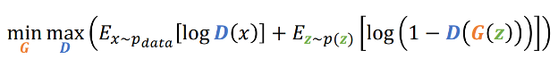
Source: [3]
D(x) represents the output from the discriminator, while G(z) represents the output from the generator. The first part tends to give a large negative number if the output of the discriminator for real data is not close to 1, while the second part gives a large negative number if the output of the discriminator for the fake data is not close to zero. By maximizing this term, the discriminator can successfully distinguish fake images from real ones. On the other hand, by minimizing this term, the generator can deceive the discriminator into considering the generated images as real ones. The generator can achieve this by making the output of D(G(z)) close to 1 for fake images. This is shown below
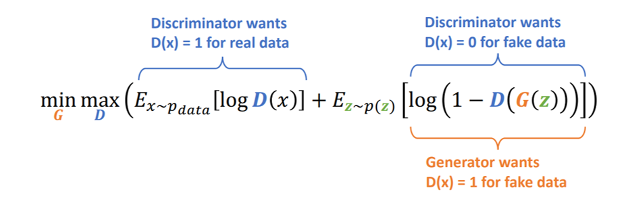
Source: [3]
Training Process
Following are the steps to train a GAN model.
- Sample x from the training dataset and z from the prior distribution and feed them to the discriminatorn and generator, respectively.
- Sample z from the prior distribution
- Feed the sampled z to generator and get the generated data.
- Feed the generated data and the real data (from step 1) to the discriminator, and get the output.
- Update both the discriminator network and the generator network. For T steps of iterations, the training process will look something like

Source: [3]
The following figure further clarify this procedure
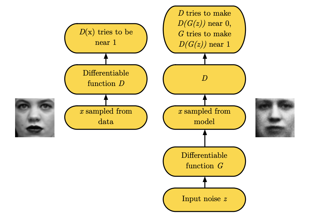
Discriminator (left) and Generator (right) - Source: [1]
A minimal code for training GAN is given below:
class Generator(nn.Module):
    def __init__(self, input_size, output_size, f):
        super(Generator, self).__init__()
        self.map1 = nn.Linear(input_size, output_size)
        self.f = f

    def forward(self, x):
        return self.f(self.map1(x))

class Discriminator(nn.Module):
    def __init__(self, input_size, output_size, f):
        super(Discriminator, self).__init__()
        self.map1 = nn.Linear(input_size, output_size)
        self.f = f

    def forward(self, x):
        return self.f(self.map1(x))

G = Generator(input_size= g_input_size, output_size=g_output_size, f=generator_activation_function)
D = Discriminator(input_size= d_input_size, output_size=d_output_size, f=discriminator_activation_function)

criterion = nn.BCELoss()
d_optimizer = optim.SGD(D.parameters(), lr=d_learning_rate, momentum=sgd_momentum)
g_optimizer = optim.SGD(G.parameters(), lr=g_learning_rate, momentum=sgd_momentum)


d_sampler = get_distribution_sampler(data_mean, data_stddev)
gi_sampler = get_generator_input_sampler()

for t in training_steps:

    D.zero_grad()
    d_real_data = d_sampler(d_input_size)
    d_real_decision = D(preprocess(d_real_data))
    d_real_error = criterion(d_real_decision, Variable(torch.ones([1])))  # ones = real data
    d_real_error.backward()


    d_gen_input = gi_sampler(minibatch_size, g_input_size)
    d_fake_data = G(d_gen_input).detach()  # detach to avoid training G on these labels
    d_fake_decision = D(preprocess(d_fake_data.t()))
    d_fake_error = criterion(d_fake_decision, Variable(torch.zeros([1])))  # zeros = fake
    d_fake_error.backward()
    d_optimizer.step()


    G.zero_grad()
    gen_input = Variable(gi_sampler(minibatch_size, g_input_size))
    g_fake_data = G(gen_input)
    dg_fake_decision = D(preprocess(g_fake_data.t()))
    g_error = criterion(dg_fake_decision, Variable(torch.ones([1])))  # Train G to pretend it's genuine

    g_error.backward()
    g_optimizer.step()  # Only optimizes G's parameters
Optimal Discriminator
Optimizing the above term from discriminator’s prospective, guarantees to reach an optimal point, only when the discriminator learns the ratio between the pdata and pmodel. We can write the loss function as
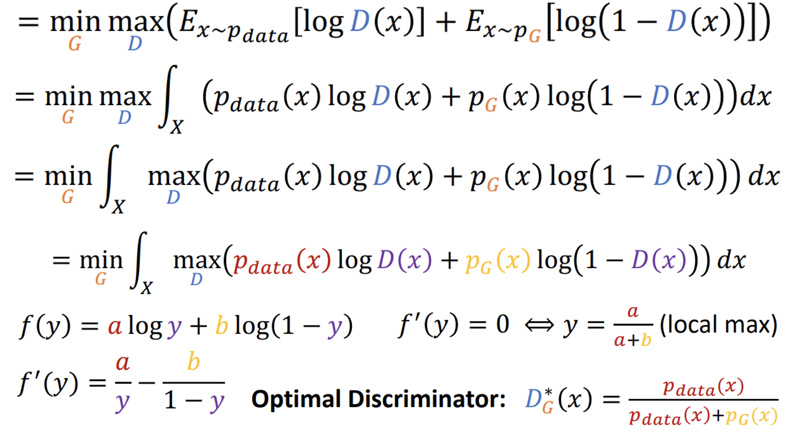
Source: [3]
The goal of the discriminator is to estimate this ratio. This is shown in the following figure

Discriminator shown in dashed blue line. The goal of the discriminator is to estimate the ratio between two distribution - Source: [1]
In order for the generator to align the pmodel distribution with the pdata, the generator distribution should move towards the direction that increases the value of D(G(z)). This also shows that the discriminator and generator are in a cooperative rather than adversarial setting, as the discriminator finds the ratio between the distributions, and then guides the generator to climb up this ratio.
Non-Saturating Game
At the beginning of the training, the discriminator gets confident about the fake images quite quickly, which causes a vanishing gradient problem for the generator. A vanishing gradient means that there will be no update for the generator, even for the bad samples. To fix this problem, we can change the equation for the generator from log(1-D(G(z))) to -log(D(G(z))). Considering a sigmoid function at the end of the discriminator network, we can see that the gradient is equal to zero at the beginning of the training. Modifying the sign reverse this phenomenon and brings the vanishing gradient problem for the real data. However, this is okay for real data, as this gradient is not used to update the generator. This is show below

The left figure shows the output of the sigmoid function and its gradient. The final layer of the discriminator is sigmoid function. The middle figure shows the default settings and the gradient under this default setting. Finally, the right most figure shows the solution to the vanishing gradient - Source: [2]
GANs and Maximum Likelihood Game
GANs models are capable of doing maximum likelhood learning. However, to achieve this, we need to minimize the KL-divergence instead of JSD between the two distributions. This can be achieved by finding such a loss function for generator whose derivative will be equal to the derivative of KL divergence.
Divergence and GANs
GAN minimizes the Jensen-Shannon divergence(JSD) between the pdata and pmodel. To prove it, we will continue the derivation from the optimal discriminator part.
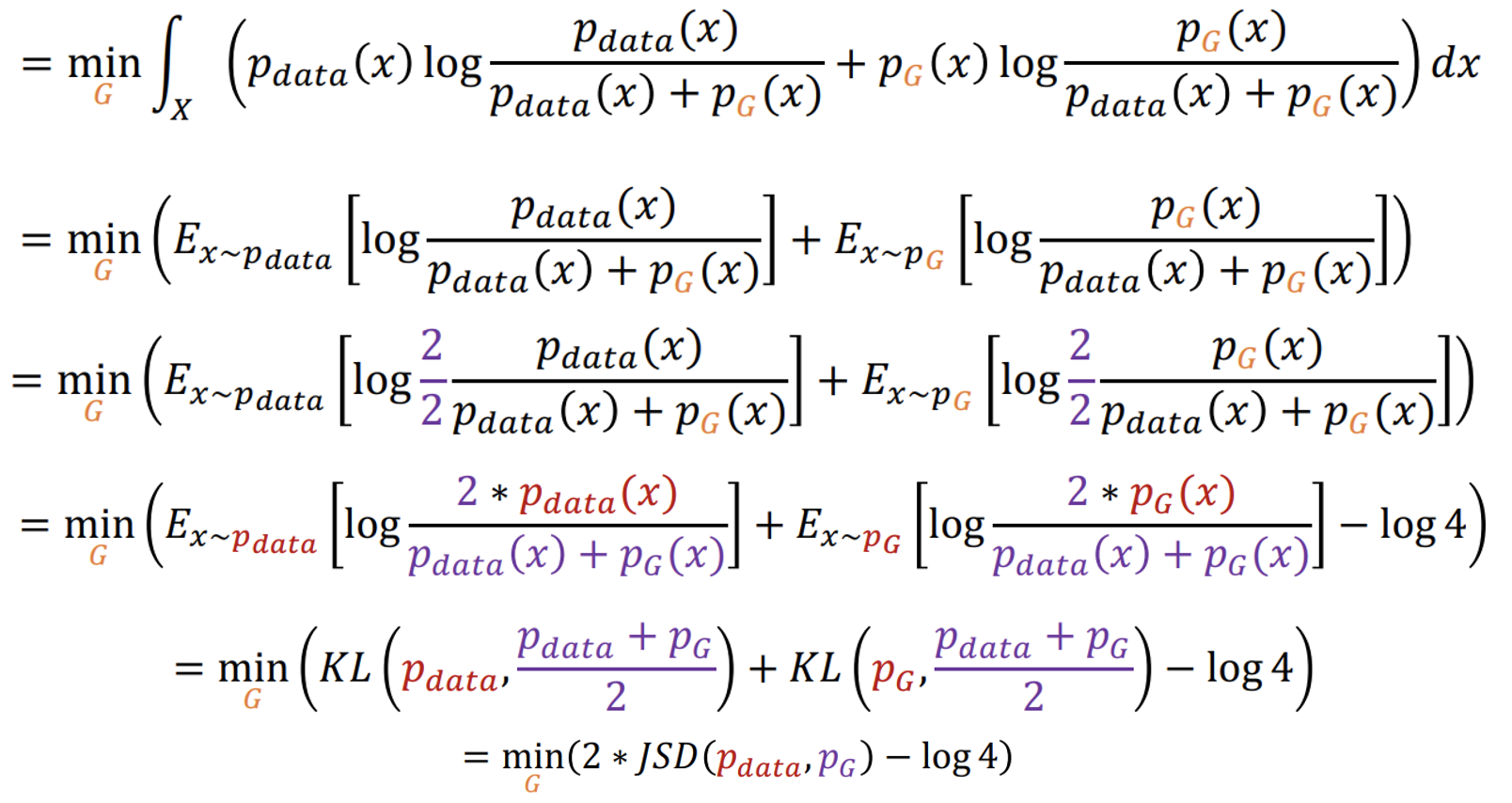
Source: [3]
We can see that minimizing the main loss function of GANs, indeed, minimizes the JSD between the two distributions. Alternatively, we can also modify the generative models to minimize the Kullback–Leibler divergence (KL) between the two distributions. This would allow the GAN to do maximum likeliood learning. In order to do so, we need to change the loss function for the generator. Specifically, changing the loss function for the generator to the following loss function will allow the GAN to minimize the KL divergence.
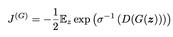
Source: [3]
Different setting results in different optimization. KL-divergence tries to fit the pmodel to all the peaks of the pdata, and therefore average out over all the modes. On the other hand, JSD tries to fit the pmodel to a single peak or model. This is shown in the following figure.
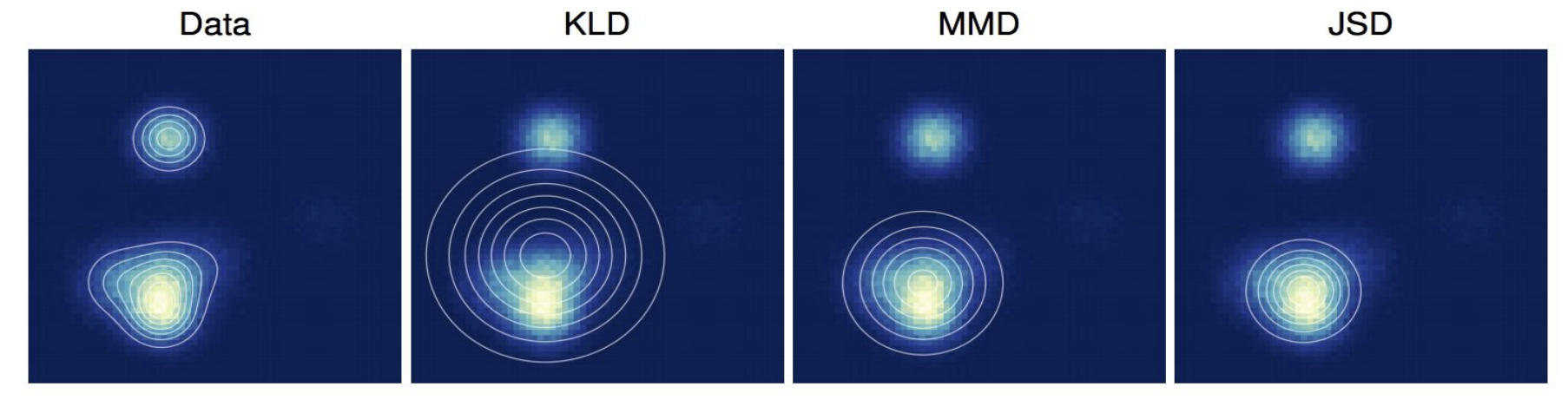
The choice of divergence defines the optimization behavior - Source: [2]
The fact that GANs try to fit pmodel to a single mode rather than averaging over multiple modes might be an explanation for why GANs produce good-quality images. However, recent efforts have shown that high quality images can also be produced by GAN when doing maximum likelihood learning.
Tips and Tricks
There are several tricks that we can use for training GANs. Some of the tricks are shown below:
Using labels to train a GAN network can improve the quality of samples generated by the model. The specific reason why providing labels works still needs to be clarified. Nonetheless, doing so improves the quality of the samples and makes them closer to the one our eyes expect the most.
If the discriminator depends only on a small sets of features to identify the real images, then the generator can easily deceive the discriminator by producing samples that have those sets of features only. This makes the discriminator overconfident for samples with specific sets of features only, even if those samples make no sense. To avoid this situation, we allow the discriminator’s output to be between 0 and 0.9. This way, even if the discriminator is sure about an image, there will be gradient for the generator to learn from. In Tensorflow, this loss can be modified as below

Source: [3]
Smoothing the labels for the fake samples will generate unexpected behaviors.
Batch Normalization (BN) creates a dependency between the samples in a batch when the size of the batch is quite small. This is problematic in GANs because when the size of the batch gets too small, the normalization constants in BN starts fluctuating. This will make the model dependent on these fluctuating constants rather than the input noise. The following figure shows this phenomenon
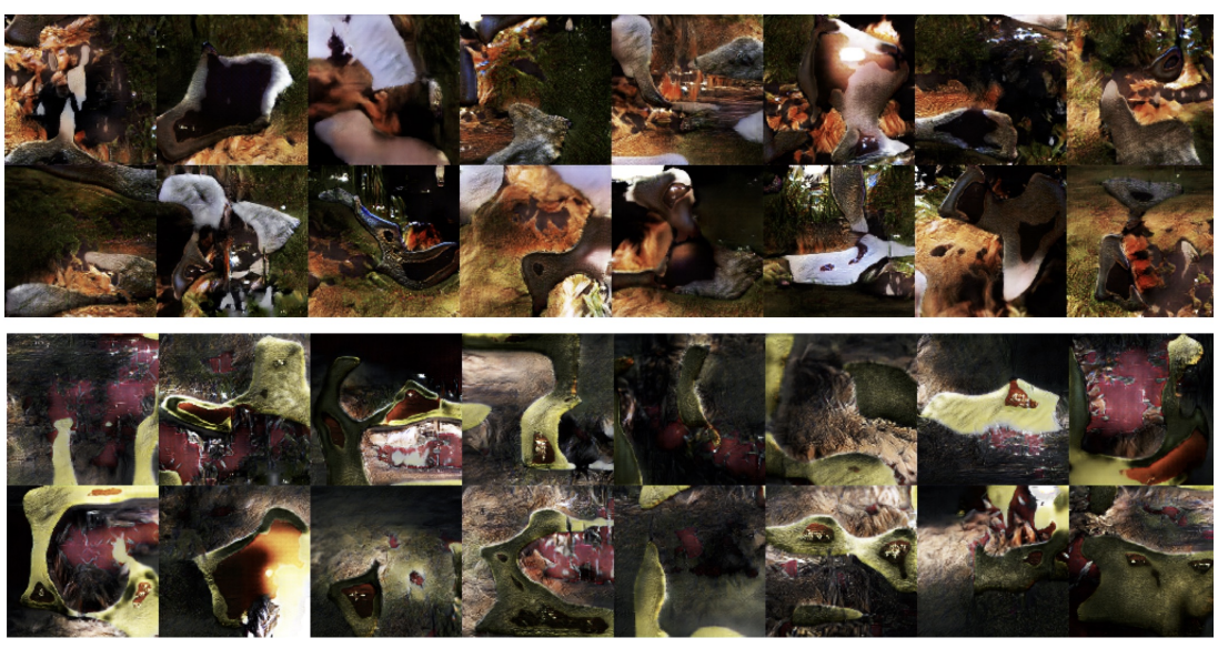
Dependence between different images in a same batch - Source:[1]
The generated images in the same batch (Two batches, top and down) are similar. Virtual batch normalization avoids this problem by sampling a reference batch before training and finding this batch’s normalization parameters. In the subsequent training steps, these normalization parameters are used together with the current batch to recompute the normalization parameters and use them during the training process.
Applications Of GANs
Generative models are of great use in real-life. Some of the examples are as follows:
- They provide a way to represent and manipulate high-dimensional probability distributions, which are quite useful in applied math and engineering.
- Reinforcement learning depends on the feedback they get from their environment. For efficiency and safety reasons, it is better to use a simulated environment than an actual one. Generative models can be used to generate the environment for the agent.
- Generative models can be used with semi-supervised learning, in which the labels for most of the data are missing. Given that semi-supervised learning can be either transductive or inductive learning, the generator models can serve as a good transductive part.
- For a given input, sometimes it is desirable to have multiple outputs. The existing approach uses MLE to average out all the possible outputs, resulting in poor results from the model. The generative model can be used to put focus on one of many possible outputs.
- Generative models are achieving state-of-the-art performance in recovering low-quality images. The knowledge of how the generative models learn actual high-resolution images is used to recover these low-quality images. Some of the other applications are image-to-image translation, text-to-image translation, image-to-text translation, and many creative projects where the goal is to create art.
The applications of generative models are not restricted to the above-mentioned ones. With more and more research coming out in this area every day, new ways are being invented to embed these models in our daily life.
Research Frontiers
Back when this paper was published, GANs were relatively new and had many research oppurtunities.
Non-convergence
The nature of the GAN settings is such that the two networks compete with each other. In simple words, one network maximizes a value while the other network minimizes the same value. This is also known as a zero-sum non-cooperative game. In game theory, GAN converges when both networks reach nash equilibrium. In nash equilibrium, one network’s actions will not affect the course of the other network’s actions. Consider the following optimization problem: minmax V(G,D) = xy
The nash equilibrium of this state reaches when x=y=0. The following figure shows the result of gradient descent on the above function.

Optimization in game theory can result in sub-optimal structure - Source: [4]
This clearly shows that some cost functions might not converge using gradient descent.
Mode Collapse
In reality, our data has multiple modes in the distribution, known as multi-modal distributions. However, sometimes, the network can only consider some of these modes when generating images. This gives rise to the problem called model collapse. In model collapse, only a few modes of data are generated.
Basically, we have two options to optimize the objective function for the GANs. One is minGmaxD V(G,D) while the other is maxDminG V(G,D)
They are different, and optimizing them corresponds to optimizing two different functions.
In the maxmin game, the generator minimizes the cost function first. It does this by mapping all the values of z to a particular x, which can be used to deceive the discriminator. And hence generator will not be learning useful mapping. On the other hand, in the minmax game, we first allow the discriminator to learn and then guide the generator to find the modes of the underlying data.
What we want the network to do is minmax; however, since we update the networks simultaneously, we end up performing maxmin. This gives rise to the mode collapse. The following figure shows this behavior
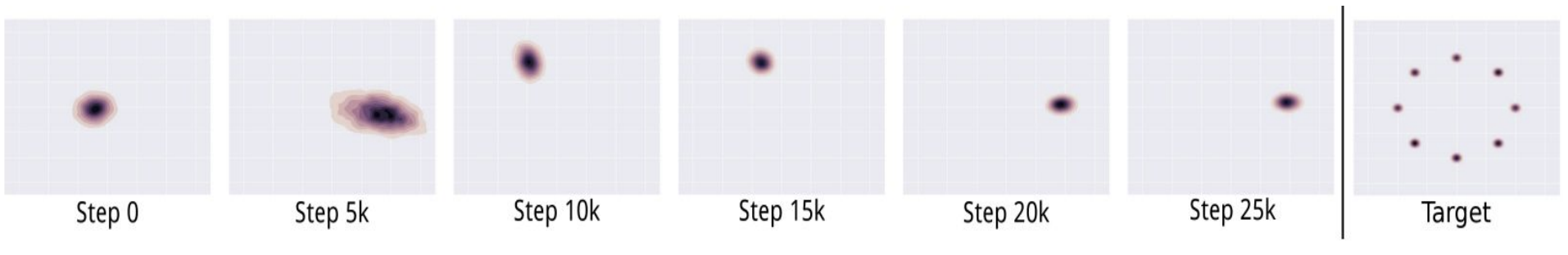
Mode collapse in toy dataset - Source: [1]
The generator visits one mode after another instead of learning to visit all different modes. The generator will identify some modes that the discriminator believes are highly likely and place all of its mass there, and then the discriminator will learn not to be fooled by going to only a single mode. Instead of the generator learning to use multiple modes, the generator will switch to a different mode, and this cycle goes on. The following note from google machine learning website best explains the cause:
"If the generator starts producing the same output (or a small set of outputs) over and over again, the discriminator's best strategy is to learn to always reject that output. But if the next generation of discriminator gets stuck in a local minimum and doesn't find the best strategy, then it's too easy for the next generator iteration to find the most plausible output for the current discriminator. Each iteration of generator over-optimizes for a particular discriminator, and the discriminator never manages to learn its way out of the trap. As a result the generators rotate through a small set of output types"
Source: Google Machine Learning
Two common methods to mitigate this problem are minibatch features and unrolled GANs.
In minibatch discrimination, we feed real images and generated images into the discriminator separately in different batches and compute the similarity of the image x with images in the same batch. We append this similarity to one of the layers in the discriminator. If the model starts to collapse, the similarity of generated images increases. This is a hint for the discriminator to use this score and penalize the generator for putting a lot of mass in one region.
Initially, when we update the networks simultaneously, we do not consider the maximized value of the discriminator for the generator. In unrolled GANs, we can train the discriminator for k steps and build the graph for each of these steps. Finally, we can propagate through all these steps and update the generator. By doing so, we can update the generator not only with respect to the loss but also with respect to the discriminator’s response to these losses. This is proved to be helpful in mode-collapse problems, as shown below.
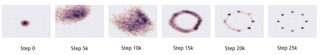
Urolled GAN solved the problem of mode collapse in toy dataset - Source [1]
You can think of unrolled GANs as a way for generator to see in the future and find out which direction the discriminator is taking it. This will help the generator not to focus on one discriminator only.
Conclusion
- GANs are type of generative models which is based upon the game theory. Specifically, in GANs, two networks compete against each other.
- GANs use supervised ratio estimation technique to approximate many cost functions, including the KL divergence used for maximum likelihood estimation.
- Training GANs require Nash equilibrium which is high dimentional, continuous, non-convex games.
- GANs are crucial to many state of the art image generation and manipulation systems and have many potentials in the future.
References
[1] Original Paper
[2] CS294
[3] Deep Learning for Computer Vision
Subscribe via RSS