VQ-VAE 블로그 정리

Introduction

VQ-VAE 이전의 VAE를 활용한 논문들은 모두 Continous하게 데이터를 표현하기 위해 Distribution을 추정합니다. VAE가 등장함으로서 우리는 빠른 Sampling과 데이터의 latent vector에 대해 더 주목할 수 있다는 장점이 있었습니다. 그러나 우리가 다루는 데이터들(Image, Audio, Video 등) 대부분은 사실 이미 Digital 상에서 표현된 데이터들입니다.

/assets/VQVAE_img/Untitled

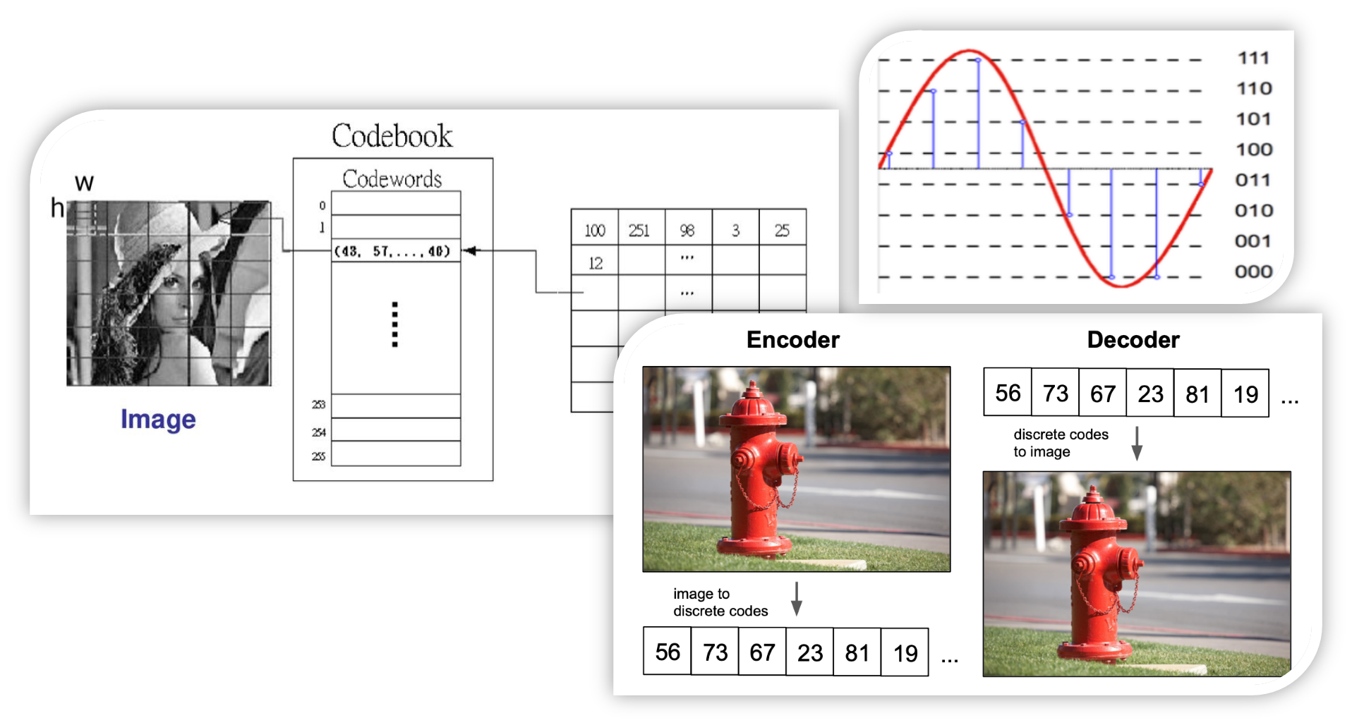
이들은 모두 Continous하게 표현되지 않고 위 그림에서 보인는 것처럼 사실은 Discrete 한 Digital number로 구성된 Dataset을 가지고 Input으로 학습하며 Output 또한 그렇게 표현을 만듭니다. 그렇기에 해당 논문에서는 Latent vector 또한 Discrete하게 표현되어야 한다고 주장합니다. 물론 과거에 이산적인 변수를 가지고 학습을 하는 것을 다른 이들이 안 떠올리지는 않았을 것입니다. 하지만 이산적인 변수는 Backprop이 불가능하여 해당 논문에서는 이산적인 표현을 살리면서 미분이 가능하도록 하는 대체 방안도 함께 제시합니다.. 이는 구조 및 loss부분에서 자세히 설명 드리겠습니다.

Ref)https://ml.berkeley.edu/blog/posts/vq-vae/

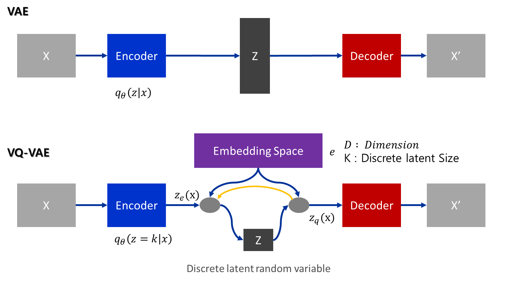
따라서 저자는 VAE와 이산 표현을 결합한 새로운 생성모델인 VQ-VAE라는 새로운 생성모델을 제안합니다. 여기서 말하는 VQ란 Vector Quantization의 약자로 VAE 구조에 VQ기능이 들어간 모델로서, 기존 VAE 구조에 Vector Quantisation(VQ)를 사용하여 기존에 continous하게 latent vector를 구성하던 것을 discrete한 latent vector로 만들어 아래와 같은 구조로 변경합니다.

/assets/VQVAE_img/Untitled

Model Structure

n : batch size
h : image height
w : image width
c : number of channels on the input image
d : number of channels in the hidden state

Processing

Reshape : 마지막 차원을 제외한 모든 차원이 하나로 결합되어 각 차원의 n×h×w 벡터를 갖습니다.
Calculating distances : n×h×w 벡터 각각에 대해 임베딩 딕셔너리의 k 벡터 각각으로부터 거리를 계산하여 (n×h×w, k) 형태의 행렬을 얻습니다.
Argmin : n×h×w 벡터 각각에 대해 사전에서 가장 가까운 k 벡터의 인덱스를 찾습니다.
Index from dictionary : n×h×w 벡터 각각에 대해 사전에서 가장 가까운 벡터를 색인화합니다.
Reshape : 다시 (n, h, w ,d) 으로 변경합니다.
Copying gradients : argmin을 통해 gradient가 흐를 수 없기 때문에 backpropagation을 통해 학습시킬 수 없습니다. 그래서 대략적으로 $z_q$의 gradient를 $z_e$에 복사해줍니다. 이 방법으로 loss function을 실제로 최소화하는 것은 아니지만 training과정에서 어느정도 정보를 줄 수 있습니다.

Vector Quantisation

posterior categorical distribution $q(z|x)$는 다음과 같이 정의됩니다.
VQVAE3

$z_e(x)$는 encoder의 output입니다.
VAE에서 $log p(x)$는 ELBO에 유계되고, VQ-VAE에서 제안된 distribution $q(z=k|x)$ 는 deterministic입니다.
simple uniform prior z를 정의함으로써, KL divergence는 상수이고 log K와 같아집니다.

VQVAE4

$z_e(x)$는 equation 1과 2에 따라서 가장 가까운 element에 매핑됩니다.

VQVAE5

모델은 입력 x로부터 받아 인코더를 통해 출력 $z_e(x)$를 생성함
Discrete latent variable z는 shared embedding space인 e로부터 가장 가까운 neighborhoodd와의 distance 계산에 의해 결정됨. 즉 가장 가까운 vector로 결정
e인 embedding space를 codebook으로 부르며, $e\ \in\ R^{K×D}$ 이며, 여기에서 K는 discrete latent space의 size가 됨(즉, K-way categorical)
D는 각각의 latent embedding vector인 $e_i$ 의 차원 수
종합적으로, K 개의 embedding vector가 존재하며, 이를 수식으로 나타내면 $e_i\ \in\ R^D,\ i\ \in\ 1, 2, …, K$ 가 됨

Loss function

Total Loss

\[L = log\ p(x|z_q(x)) + ||sg[z_e(x)]-e||_2^2\ + \beta||z_e(x)-sg[e]||_2^2\]

sg : stopgradient operator
Decoder는 첫번째 loss term에서만 optimize됩니다
Encoder는 첫번째 세번째 loss term에서 optimize됩니다
Embedding은 중간 loss term에 의해 optimize됩니다
VQ-VAE는 z에 대해 uniform prior를 가정하기 때문에, 일반적으로 ELBO에 나타나는 KL term은 상수입니다. encoder parameter는 training과정에서 무시할 수 있습니다.

Reconstruction Loss

\[L = log\ p(x|z_q(x))\]

Reconstruction Loss : which optimizes the decoder and encoder

\[z_q(x) = e_k, \quad where \quad k=argmin_j||z_e(x)-e_j||_2 \qquad (2)\]

equation 2에서 real gradient가 없습니다
decoder input $z_q(x)$에서 encoder output $z_e(x)$로 그냥 gradient를 복사합니다.

Codebook Loss

\[L = ||sg[z_e(x)]-e||_2^2\]

Codebook Loss : gradient가 embedding을 우회하기 때문에, L2 error를 사용하여 embedding vector를 이동하는 dictionary learning algorithm을 사용합니다. $e_i$은 encoder output 방향으로 업데이트됩니다

이 loss term은 dictionary를 update하는 것에만 사용됩니다

Commitment Loss

\[L = \beta||z_e(x)-sg[e]||_2^2\]

Commitment Loss : since the volume of the embedding space is dimensionless, it can grow arbirtarily if the embeddings $e_i$ do not train as fast as the encoder parameters, and thus we add a commitment loss to make sure that the encoder commits to an embedding

$\beta$를 0.1부터 2.0까지 다양하게 두고 실험을 진행하였지만 결과는 크게 다르지 않고 robust했습니다.
VQ-VAE에서는 모든 실험에 $\beta$ = 0.25를 사욯했습니다
** 일반적으로 이것은 reconstruction loss의 scale에 따라 달라집니다

Log-likelihood of the complete model

\[log\ p(x) = log\ \sum_k d=p(x|z_k)p(z_k)\]

MAP-inference에서 decoder $p(x z)는\ z = z_q(x)$이기 때문에
완전히 수렴되면 decoder는 $z \ne z_q(x)$인 $p(x|z)$가 존재하지 않게 됩니다.
따라서
-> $ log\ p(x) \approx log\ p(x|z_q(x))p(z_q(x))$
-> $ log\ p(x) \ge log\ p(x|z_q(x))p(z_q(x))$ (Jensen’s inequality)

Posterior Collapse

posterior collapse는 왜 발생할까요?

decoder가 latent z 없이 과거 데이터로만 충분히 생성할 수 있는 경우
가정한 Gaussian prior가 사실 정보를 줄 수 없는 경우(가정이 잘못됨)
ELBO와 evidence간의 차이, true posterior approximation의 실패
encoder가 training 초기에 의미있는 z를 표현하지 못하기 때문

VQVAE6

근사된 posterior는 prior를 흉내내고 model은 latent variable을 무시하면서 학습을 진행된다는 것을 의미합니다.

PixelCNN Prior

latent p(z)는 categorical distribution이라서 latent z를 feature map으로 하여 autoregressive 모델을 만들 수 있습니다. 그래서 학습된 TVQ-VAE의 latent z를 condition으로 하여 PixelCNN이 이미지를 생성하도록 할 수 있습니다.
VQ-VAE를 학습한 후에, PixelCNN에서 image에서 discrete latent를 만들도록 학습합니다. pre-trained PixelCNN에서 생성된 discrete latent vector는 VQ-VAE decoder의 input으로 들어가서 이미지를 생성합니다.

Experiments

저자는 VQ-VAE를 통해 데이터를 Vector Quantization하게 표현하여 학습을 시킴으로써 성능이 월등히 높아졌다는 표현을 하지 않습니다. 오히려 아래와 같이 “Vector quantization으로 Latent를 표현하면 VAE만큼 성능이 나오더라 “라고 합니다.

/assets/VQVAE_img/Untitled

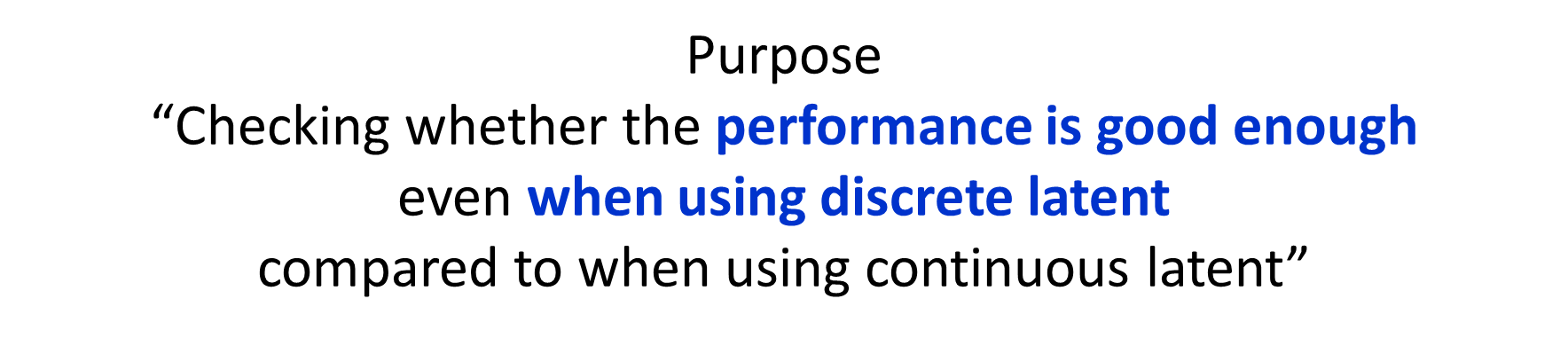
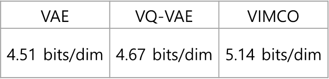
실제로 결과 또한 아래와 같이 기존 VAE와 좀 떨어지고 Monte Carlo 방법으로 생성한 VIMCO보다는 좋은 성능 결과를 제시합니다.

/assets/VQVAE_img/Untitled

하지만 이미지 자체를 눈으로 보게되면, 그래도 VAE보다는 그럴듯한 그림을 만들어낸다는 것을 알 수 있습니다. 아래 사진에서 배 모양 그림을 보면 Detail 한 영역에서는 알수 없는 그림을 내놓는 것도 확인 할 수 있습니다.

/assets/VQVAE_img/Untitled

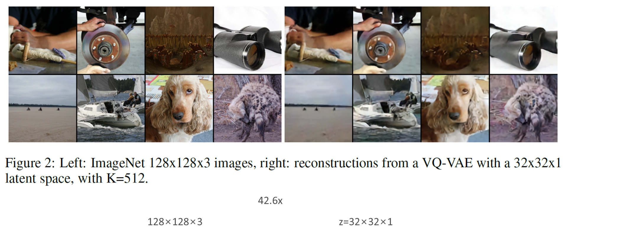
위 실험의 경우 차원을 128x128x3에서 z를 32x32x1 까지 42.6 배를 축소하였음에도 이미지의 중요한 정보를 잃지 않음을 알 수 있었습니다.

/assets/VQVAE_img/Untitled

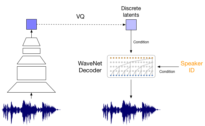
또한 음성에 대해서도 실험을 진행하였는데, VQ-VAE를 오직 long-term 상관관계(정보)만을 보존하도록 latent space를 만든 뒤 decoder로 복원하는 작업을 수행하였습니다. 예시를 들어보면 알 수 있겠지만, 그 내용은 변하지 않았으나 운율은 상당히 바뀐 것을 들을 수 있습니다. 이는 VQ-VAE가 어떤 언어적 지도 없이 고수준의 추상 공간을 이해하고 중요하지 않은 부분은 버리며 음성의 내용만을 잡아냈음을 뜻합니다.

위에 음성이 Original, 아래 음성이 Reconstruction한 음성입니다.

Test A:

https://avdnoord.github.io/homepage/audio/pt1_orig1.wav

https://avdnoord.github.io/homepage/audio/pt1_recon1.wav

Test B:

https://avdnoord.github.io/homepage/audio/pt1_orig2.wav

https://avdnoord.github.io/homepage/audio/pt3_transfer2.wav

Test C:

https://avdnoord.github.io/homepage/audio/pt3_source3.wav

https://avdnoord.github.io/homepage/audio/pt3_transfer3.wav

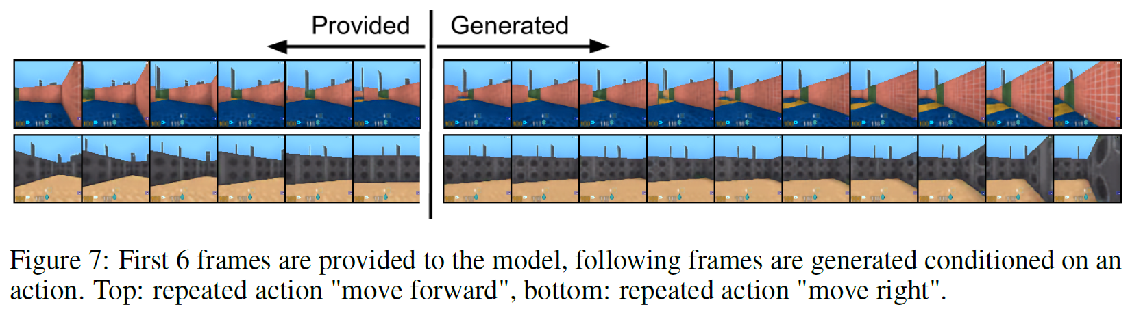
Video에서도 실험을 진행하였는데, DeepMind Lab 환경에서 처음 6 frame이 주어지면 나머지 10 frame을 이어지는 내용으로 채우는 task로, 여기서 VQ-VAE가 하는 것은 오직 latent space(z_t) 상에서만 생성할 뿐 이미지를 직접 생성하지 않습니다.

sequence xi안의 각 이미지는 prior model만 사용하여 모든 latent를 생성한 후 deterministic decoder로 대응되는 latent와 mapping시켜서 생성하게 됩니다. 따라서 VQ-VAE는 latent space 안에서만 수행하고 pixel space에서는 작업하지 않는다. 생성 결과는 아래 그림과 같습니다.

/assets/VQVAE_img/Untitled

Conclusion

VAE와 discrete latent 표현을 위한 VQ를 결합하여 새로운 생성 모델을 만들었습니다.
VQ-VAE는 long-term dependency를 잘 모델링할 수 있습니다.
원본 source를 작은 latent로 수십 배 압축할 수 있습니다.
이러한 latent는 discrete하며, continuous latent와 비교하여 성능이 필적할 만합니다.
Image, audio, video 모두에 대해서 잘 모델링 및 압축한 후 중요한 내용을 잘 보존하면서 복원이 가능합니다.

Future Work

/assets/VQVAE_img/Untitled

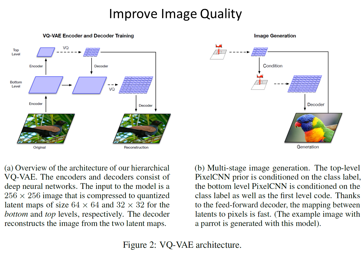
Image Experiment때 보았지만, 음성에서는 탁월한 성능을 내지만 디테일한 영역에서는 아직 표현이 어렵습니다. 따라서 이 이미지에 특화된 VQ-VAE모델을 만든것이 VQ-VAE2입니다.

VQ-VAE2는 Large scale 이미지 생성 문제에 집중한 모델로, prior를 더욱 강화하여 이전 보다 더 일관성, 현실성 있는 이미지 생성합니다. 해당 이미지 결과는 그럴듯한 이미지를 만들기로 유명한 GAN과 비슷한성능을 냅니다. 핵심적인 내용은 VQ-VAE와 다르게 더 큰 이미지를 다룰 수 있기 위해 vector quantized codes를 계층 구조로 사용한다는 것입니다. 먼저, Bottom latent code에서 세부적인 부분을 모델링하고 bottom latent code를 한번 더 인코딩한 Top latent code는 global한 특징을 모델링함으로써 이미지 Feature을 더 잘 표현하게 만듭니다.

Quantization Code

  class VectorQuantizer(nn.Module):
    """
    Discretization bottleneck part of the VQ-VAE.
    Inputs:
    - n_e : number of embeddings
    - e_dim : dimension of embedding
    - beta : commitment cost used in loss term, beta * ||z_e(x)-sg[e]||^2
    """

    def __init__(self, n_e, e_dim, beta):
        super(VectorQuantizer, self).__init__()
        self.n_e = n_e
        self.e_dim = e_dim
        self.beta = beta

        self.embedding = nn.Embedding(self.n_e, self.e_dim)
        self.embedding.weight.data.uniform_(-1.0 / self.n_e, 1.0 / self.n_e)

    def forward(self, z):
        """
        Inputs the output of the encoder network z and maps it to a discrete 
        one-hot vector that is the index of the closest embedding vector e_j
        z (continuous) -> z_q (discrete)
        z.shape = (batch, channel, height, width)
        quantization pipeline:
            1. get encoder input (B,C,H,W)
            2. flatten input to (B*H*W,C)
        """
        # reshape z -> (batch, height, width, channel) and flatten
        z = z.permute(0, 2, 3, 1).contiguous()
        z_flattened = z.view(-1, self.e_dim)
        # distances from z to embeddings e_j (z - e)^2 = z^2 + e^2 - 2 e * z

        d = torch.sum(z_flattened ** 2, dim=1, keepdim=True) + \
            torch.sum(self.embedding.weight**2, dim=1) - 2 * \
            torch.matmul(z_flattened, self.embedding.weight.t())

        # find closest encodings
        min_encoding_indices = torch.argmin(d, dim=1).unsqueeze(1)
        min_encodings = torch.zeros(
            min_encoding_indices.shape[0], self.n_e).to(device)
        min_encodings.scatter_(1, min_encoding_indices, 1)

        # get quantized latent vectors
        z_q = torch.matmul(min_encodings, self.embedding.weight).view(z.shape)

        # compute loss for embedding
        loss = torch.mean((z_q.detach()-z)**2) + self.beta * \
            torch.mean((z_q - z.detach()) ** 2)

        # preserve gradients
        z_q = z + (z_q - z).detach()

        # perplexity
        e_mean = torch.mean(min_encodings, dim=0)
        perplexity = torch.exp(-torch.sum(e_mean * torch.log(e_mean + 1e-10)))

        # reshape back to match original input shape
        z_q = z_q.permute(0, 3, 1, 2).contiguous()

        return loss, z_q, perplexity, min_encodings, min_encoding_indices
  
  